[텐서플로우/케라스] MNIST 숫자 분류하기 (softmax)
2020. 4. 21. 12:55ㆍ노트/Python : 프로그래밍

텐서플로우
데이터 불러오기
import tensorflow as tf
import matplotlib.pyplot as plt
import random

tf.set_random_seed(777)
from tensorflow.examples.tutorials.mnist import input_data

mnist =input_data.read_data_sets("MNIST_data/", one_hot=True)
변수 정의
x = tf.placeholder(tf.float32, [None,784])
y = tf.placeholder(tf.float32, [None,10]) # 0~9 digit
w = tf.Variable(tf.random_normal([784,10]))
b = tf.Variable(tf.random_normal([10]))
함수 및 모델 정의
hf = tf.nn.softmax(tf.matmul(x,w)+b)
cost = tf.reduce_mean(-tf.reduce_sum( y * tf.log(hf) ,axis=1))
train = tf.train.GradientDescentOptimizer(0.1).minimize(cost)

isCorrect = tf.equal(tf.argmax(hf ,1) , tf.argmax(y,1))
accuracy = tf.reduce_mean(tf.cast(isCorrect , tf.float32 ))

numEpochs = 15
batchSize = 100
numIter = int(mnist.train.num_examples / batchSize )
모델 실행
with tf.Session() as sess:
    sess.run(tf.global_variables_initializer())
    #트레이닝
    for epoch in range(numEpochs): #15에폭
        avgCv = 0
        for i in range(numIter): #600반복
            batchX, batchY = mnist.train.next_batch(batchSize)
            _, cv = sess.run([train, cost], feed_dict={x:batchX, y:batchY})
            avgCv += cv / numIter
        print("epoch:{:04d}, cost:{:.9f}".format(epoch+1, avgCv)) # 4자리수로 출력
    print("정확도:",accuracy.eval(session=sess, feed_dict={x:mnist.test.images, y:mnist.test.labels}))
    r=random.randint(0,mnist.test.num_examples-1) #난수발생
    print("레이블:",sess.run(tf.argmax(mnist.test.labels[r:r+1],1)))
    print("예측:",sess.run(tf.argmax(hf,1),feed_dict={x:mnist.test.images[r:r+1]}))

    plt.imshow(mnist.test.images[r:r+1].reshape(28,28),cmap="Greys")
    plt.show()

 >>>
 epoch:0001, cost:2.826302752
epoch:0002, cost:1.061668976
epoch:0003, cost:0.838061328
epoch:0004, cost:0.733232746
epoch:0005, cost:0.669279894
epoch:0006, cost:0.624611839
epoch:0007, cost:0.591160358
epoch:0008, cost:0.563868996
epoch:0009, cost:0.541745189
epoch:0010, cost:0.522673595
epoch:0011, cost:0.506782334
epoch:0012, cost:0.492447652
epoch:0013, cost:0.479955845
epoch:0014, cost:0.468893677
epoch:0015, cost:0.458703488
정확도: 0.8951
레이블: [6]
예측: [6]
케라스
# 학습 모델 저장 / 불러오기 (keras)
# 다층 퍼셉트론 모델 (히든 레이어 여러개 생성)
# 훈련셋, 검증셋, 시험셋
데이터준비
from keras.utils import np_utils
from keras.datasets import mnist
from keras.models import Sequential
from keras.layers import Dense , Activation
import numpy as np

(xTrain, yTrain),(xTest,yTest) = mnist.load_data()
# 전처리작업 (스케일링)
xTrain=xTrain.reshape(60000,784).astype('float32')/255.0
xTest=xTest.reshape(10000,784).astype('float32')/255.0

yTrain=np_utils.to_categorical(yTrain) # 원핫인코딩
yTest=np_utils.to_categorical(yTest) # 원핫인코딩

# 검증데이터 나누기
xVal=xTrain[42000:]
xTrain=xTrain[:42000]  # 순서주의 Val 부터 먼저뽑아야함
yVal=yTrain[42000:]
yTrain=yTrain[:42000]
모델구축
# 모델 구성
model = Sequential()
model.add(Dense(units=64, input_dim=28*28, activation="relu"))
model.add(Dense(units=10, activation="softmax"))

# 모델 학습
# 모델 학습환경설정 (compile)
model.compile(loss= "categorical_crossentropy", optimizer = "sgd", metrics=["accuracy"])
# 모델 학습 (fit)
model.fit(xTrain,yTrain,epochs=5,batch_size=50, validation_data=(xVal,yVal))

# 모델평가하기(test data)
metrics = model.evaluate(xTest,yTest,batch_size=50)
print("평가결과:"+str(metrics))

>>10000/10000 [==============================] - 0s 13us/step
평가결과:[0.2885529683995992, 0.9204000234603882]
모델사용
# 모델 예측하기
idx = np.random.choice(xTest.shape[0],5)
xHat = xTest[idx]
yHat = model.predict_classes(xHat)

for i in range(5):
    print("예측값:", str(yHat[i]) + " 실제값:"+str(np.argmax(yTest[idx[i]])))

>>>
예측값: 7 실제값:7
예측값: 1 실제값:1
예측값: 9 실제값:4
예측값: 3 실제값:3
예측값: 2 실제값:2
# 모델 아키텍쳐 확인
from keras.utils.vis_utils import model_to_dot
from IPython.display import SVG

model.summary()
케라스 기반 성능 향상
- optimizer = sgd > adam
- validation data = test data
데이터 불러오기
from keras.datasets import mnist
from keras.utils import np_utils
import numpy as np
import sys
import tensorflow as tf

(xTrain, yTrain ), (xTest, yTest)= mnist.load_data()

print(xTrain.shape)
print(yTrain.shape)
print(xTest.shape)
print(yTest.shape)
>>>
(60000, 28, 28)
(60000,)
(10000, 28, 28)
(10000,)

import matplotlib.pyplot as plt

plt.imshow(xTrain[0], cmap="Greys")
plt.show()
for x in xTrain[0]:
for i in x:
sys.stdout.write("%d\t" % i)
sys.stdout.write("\n") #표준출력장치 (모니터)로 출력하여라
yTrain[0]
>>> 5

#원핫인코딩
yTrain=np_utils.to_categorical(yTrain,10)
yTest=np_utils.to_categorical(yTest,10)
모델 구성
from keras.models import Sequential
from keras.layers import Dense
from keras.callbacks import ModelCheckpoint, EarlyStopping
import numpy as np
import tensorflow as tf
import os

# 모델 구성
model = Sequential()
model.add(Dense(512, input_dim = 784, activation = 'relu')) # 출력이 512개인 layers
model.add(Dense(10, activation = 'softmax'))

# 모델 환경설정
model.compile(loss="categorical_crossentropy",
             optimizer = "adam",
             metrics=['accuracy'])

# 모델 최적화
modelDir = './myModel/'
if not os.path.exists(modelDir):  # 만약 myModel directory가 존재하지 않는다면
    modelPath = "./myModel/{epoch:02d}-{val_loss:.4f}.hdf5"
    os.mkdir(modelDir)
checkpointer = ModelCheckpoint(filepath=modelPath, monitor = 'val_loss', verbose=1 , save_best_only=True )
# ModelCheckpoint: 콜백함수 : 어떤 상황이 되면 시스템에 의해서 호출되는 함수 ,
# keras에서 모델을 학습할 때마다 중간중간에 콜백형태로 알려줌
# save_best_only: 모델의 정확도가 최고값을 갱신할때만 저장
es = EarlyStopping(monitor='val_loss', patience=10)
모델 실행
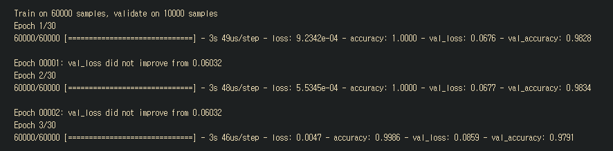
history= model.fit(xTrain, yTrain,validation_data=(xTest,yTest),
                   epochs=30, batch_size=200, callbacks=[es,checkpointer])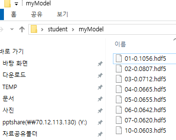
모델 평가
print("테스트 정확도: %.4f" %(model.evaluate(xTest,yTest)[1]))

10000/10000 [==============================] - 0s 40us/step
테스트 정확도: 0.9813
# 테스트 셋의 오차
yVloss = history.history['val_loss']
# 학습 셋의 오차
yLoss=history.history['loss']

%matplotlib notebook
xLen = np.arange(len(yLoss))
plt.plot(xLen, yVloss, marker=".", c="red", label="testset_loss")
plt.plot(xLen, yLoss, marker=".", c="blue", label="trainset_loss")
plt.legend()
plt.grid()
plt.xlabel('epoch')
plt.ylabel('loss')
plt.show()
'노트 > Python : 프로그래밍' 카테고리의 다른 글
| [파이썬] 데이터시각화(2) (seaborn 패키지) (0) | 2020.04.22 |
|---|---|
| [신경망] 선형회귀로 분류가 불가능한 경우(XOR problem) (0) | 2020.04.21 |
| [텐서플로우] 소프트맥스 회귀 (Softmax Regression) 분류 파이썬 코드 (0) | 2020.04.20 |
| [파이썬] 데이터시각화(1) (matplotlib.pyplot 패키지) (0) | 2020.04.20 |
| [케라스] 주식가격 예측하기(2) 파이썬 코드 (0) | 2020.04.18 |