2021. 8. 2. 18:17ㆍ노트/Python : 프로그래밍
https://towardsdatascience.com/attention-in-computer-vision-fd289a5bd7ad
Attention in computer vision
Ever since the introduction of Transformer in the work “Attention is all you need”, there has been a transition in the field of NLP towards replacing Recurrent Neural Networks (RNN) with…
towardsdatascience.com
Attention in computer vision
MultiHead 와 CBAM attention 모듈 PyTorch로 구현하기

"Attention is all you need"라는 Transformer 연구의 도입 이후로, 순환신경망 (RNN) 을 어텐션 기반의 네트워크로 대체하고자 하는 NLP 분야의 변화가 있어왔다. 현재 문헌에서는, 이 방법을 묘사한 많은 아티클들이 있다. 지금까지 내가 본 리뷰 중에, 가장 좋았던 두가지를 소개하겠다. : The Annotated Transformer 와 Transformers explained Visually .
하지만, attention을 computer vision에 어떻게 구현하는지 연구한 이후로, ( Best로 알려진 articles들 : Understanding Attention Modules , CBAM , Papers with Code-Attention, Self-Attention, Self-Attention and Conv , ) 이 중에 몇개만 attention 메커니즘을 정확하게 설명하고 이론과 함께 clean code를 포함한다는 것을 알게 되었다. 그래서, 이번 article의 목표는 컴퓨터 비젼에서 가장 중요한 두가지 attention 모듈을 설명하고, PyTorch를 사용해서 실제 케이스에 적용해보는 것이다. 이번 아티클의 구조는 다음과 같다 :
1. 어텐션 모듈 소개
2. 컴퓨터 비젼에서의 어텐션 기법
3. 어텐션 기반의 네트워크 실행과 결과
4. 결론
1. 어텐션 모듈 소개
머신러닝 맥락에서, attention은 주의를 인식하는 것, 즉 관련된 자극에 집중하고 선택하는 능력, 을 모방한 기법입니다. 다른 말로, attention은 관련 없는 정보를 잊어버리면서 중요한 부분에 집중하려고 노력하는 기법입니다.
비록 이 메커니즘이 두가지 집단(Attention? Attention! )으로 구분됨에도 불구하고, 우리는 self-attention기법에 집중하려고하며, 이유는 컴퓨터 비젼 task에서 가장 유명한 어텐션 유형이기 때문이다. 이것은 동일한 시퀀스의 표현을 계산하기 위해, 단일 시퀀스의 서로 다른 위치를 연관시키는 메커니즘을 말합니다.
이 개념을 더 잘 이해하기 위해서, 다음 문장을 생각해봅시다 : Bank of a river (강둑). 만약 우리가 River를 볼 수 없다면, Bank라는 단어는 문맥적인 정보를 잃게 된다는 것에 동의하나요? 이것이 self-attention의 메인 아이디어입니다.
각 단어의 의미가 문장 속에서의 의미를 나타내는 것이 아니기 때문에, self-attention은 각 단어의 문맥적인 정보를 주려고 노력합니다. An Intuitive Explanation of Self-attention에 설명이 되어있듯이, 만약 위에서 말한 예시를 고려해본다면, self-attention은 문장 속의 모든 단어를 다른 단어들과 비교하고, 문맥적 연관성을 포함하는 각 단어들의 단어 임베딩을 reweighting 하면서 작동합니다. 모듈을 출력하기 위한 input은 각 단어들의 문맥적 정보들이 없는 embedding 값들이며, output은 문맥적 정보가 포함된 유사한 embedding 입니다.
2. 컴퓨터 비젼에서의 어텐션 기법
여기에 어텐션 모듈에 대해서 계속적으로 업데이트된 리스트가 있습니다. 한 리스트로 부터, 컴퓨터 비젼 테스크에서 가장 유명한 두가지에 집중해보겠습니다 : Multi-Head Attention 과 Convolutional Block Attention Module (CBAM) 입니다.
2.1 Multi-Head Attention
Multi-Head Attention은 어텐션 모듈을 몇번 병렬로 처리하는 어텐션 메커니즘 모듈입니다. 그래서, 이 로직을 이해하기 위해, 처음으로 Attention 모듈을 이해해야 합니다. 두가지 가장 공통적으로 사용되는 어텐션 함수는 Additive Attention과 Dot-Product Attention이며, 이번 연구에서는 후자에 더 관심이 있습니다.
Attention 모듈의 기본적인 구조는 벡터 x1과 x2의 두개의 리스트가 있다는 점입니다. 하나는 attend 된 것이고 다른 하나는 attend할 것입니다. 벡터 x2는 'query'를 만드는 반면, 벡터 x1은 'key'와 'value'를 만듭니다. 어텐션 함수의 아이디어는 query와 출력될 key-value 쌍을 매핑하는 것입니다. "output은 각 value에 할당된 가중치는 해당 key와 query의 호환되는 함수로 계산된 value들의 가중합으로 계산됩니다. " [Attention is all you need]. output은 다음과 같이 계산됩니다.
이 discussion 에서 언급되었듯이, key/value/query 개념은 검색 시스템에서 유래되었습니다. 예를들어, 몇몇 비디오를 찾기 위해, Youtube에 쿼리를 입력햇을때, 검색 엔진은 당신의 query를 데이터베이스의 후보 비디오들의 링크 키 (keys) 세트 (video title, description, 등) 에 대해 매핑합니다. 그리고나서, 당신에게 최적으로 매칭된 비디오 (values) 를 제시합니다.
이 Multi-Head attention으로 이동하기 전에 이 모듈의 확장판인 Dot-Product Attention을 실행해봅시다. 아래는 PyTorch로 구현되었습니다. input 사이즈는 [128, 32, 1, 256] 입니다. 128은 batch에 해당하고, 32는 시퀀스 길이를, 1은 heads 갯수를 (multiple attention heads 에서는 늘릴 것입니다.) 그리고 256은 feature 갯수를 각각 의미합니다.
import torch
import torch.nn as nn
import torch.nn.functional as F

# Input : [128,32,1,256]
# 128 : batch
# 32 : sequence length
# 1 : n of heads
# 256 : n of features

class ScaledDotProductAttention(nn.Module):
    """ Scaled Dot-Product Attention """
    def __init__(self, key_dimension, attn_dropout = 0.0):
        super().__init__()
        self.key_dimension = key_dimension
        self.dropout = nn.Dropout(attn_dropout)
        # temperature 는 무슨 기능??
    def forward(self, q, k , v , mask = None):
        attn = torch.matmul(q / self.key_dimension, k.transpose(2,3)) # k : [128,1,32,256]
        if mask is not None :
            attn = attn.masked_fill(mask == 0, -1e9)
        attn = self.dropout(F.softmax(attn, dim=-1))
        output = torch.matmul(attn, v)
        return output, attn

# Attention
query = torch.rand(128,32,1,256)
key = value = torch.rand(128,16,1,256) # 왜 16???
query, key, value = query.transpose(1,2) , key.transpose(1,2), value.transpose(1,2)
multihead_attn = ScaledDotProductAttention(key_dimension = key.size(2))
attn_output , attn_weights = multihead_attn(query, key, value)
attn_output = attn_output.transpose(1,2)
print(f'attn_output: {attn_output.size()}, attn_weights: {attn_weights.size()}')

# Self-attention
query = torch.rand(128,32,1,256)
query = query.transpose(1,2)
multihead_attn = ScaledDotProductAttention(key_dimension = query.size(2))
attn_output, attn_weights = multihead_attn(query, query, query)
attn_output = attn_output.transpose(1,2)
print(f'attn_output: {attn_output.size()}, attn_weights: {attn_weights.size()}')


>>> attn_output: torch.Size([128, 32, 1, 256]), attn_weights: torch.Size([128, 1, 32, 16])
    attn_output: torch.Size([128, 32, 1, 256]), attn_weights: torch.Size([128, 1, 32, 32])
이 기본 구현으로 부터 몇가지 이점들이 있습니다. :
- output은 query input size와 같은 shape을 가집니다.
- 각 데이터에 대한 attention weights는 행렬을 가지며, 여기서 행(row)의 수는 query의 sequence 길이에 상응하며, 열(columns)의 수는 key의 sequence 길이에 상응합니다.
- Dot-Product Attention에는 학습가능한 파라미터가 없습니다.
그럼, Multi-Head Attention으로 돌아오면, 이 Multi-Head Attention은 설명한 Attention 모듈을 몇번 병렬로 실행합니다. 독립적인 attention outputs은 그리고나서 결합되고, 예상된 차원으로 선형적으로 변환됩니다. 여기에 구현된 코드가 있습니다. :
class MultiHeadAttention(nn.Module):
    """ Multi-Head Attention module """
    def __init__(self, n_head, d_model, d_k, d_v, dropout = 0.1):
        super().__init__()
        self.n_head = n_head
        self.d_k = d_k
        self.d_v = d_v

        self.w_qs = nn.Linear(d_model, n_head * d_k , bias = False)
        self.w_ks = nn.Linear(d_model, n_head * d_k , bias = False)
        self.w_vs = nn.Linear(d_model, n_head * d_v , bias = False)
        self.fc = nn.Linear(n_head * d_v, d_model, bias = False)

        self.attention = ScaledDotProductAttention(key_dimension = d_k ** 0.5)

        self.dropout = nn.Dropout(dropout)
        self.layer_norm = nn.LayerNorm(d_model, eps = 1e-6)

    def forward(self, q, k, v, mask = None):
        d_k, d_v, n_head = self.d_k, self.d_v, self.n_head
        sz_b, len_q, len_k, len_v = q.size(0), q.size(1), k.size(1), v.size(1)
        residual = q

        # Pass through the pre-attention projection: b x 1q x (n*dv)
        # Separate different heads: b x 1q x (n * dv)
        q = self.w_qs(q).view(sz_b, len_q, n_head , d_k )
        k = self.w_ks(k).view(sz_b, len_k, n_head , d_k )
        v = self.w_vs(v).view(sz_b, len_v, n_head , d_v )

        # Transpose for attention dot product : b x n x 1q x dv
        q, k, v = q.transpose(1,2) , k.transpose(1,2) , v.transpose(1,2)

        if mask is not None:
            mask = mask.unsqueeze(1) # For head axis broadcasting.
        q, attn = self.attention(q, k, v, mask = mask)

        # Transpose to move the head dimension back: b x 1q x n x dv
        # Combine the last two dimensions to concatenate all the heads together: b x 1q x (n*dv)
        q = q.transpose(1,2).contiguous().view(sz_b, len_q, -1)
        q = self.dropout(self.fc(q))
        q += residual

        q = self.layer_norm(q)
        return q, attn

query = torch.rand(128,32,256)
multihead_attn = MultiHeadAttention(n_head = 8, d_model = 256, d_k = 32, d_v = 32)
attn_output, attn_weights = multihead_attn(query, query, query)
print(f'attn_output: {attn_output.size()}, attn_weights: {attn_weights.size()}')

query = torch.rand(128,32,256)
multihead_attn = MultiHeadAttention(n_head = 8, d_model = 256, d_k = 256, d_v = 512)
attn_output, attn_weights = multihead_attn(query,query,query)
print(f'attn_output: {attn_output.size()}, attn_weights: {attn_weights.size()}')

>>> attn_output: torch.Size([128, 32, 256]), attn_weights: torch.Size([128, 8, 32, 32])
    attn_output: torch.Size([128, 32, 256]), attn_weights: torch.Size([128, 8, 32, 32])
코드로부터, 다음을 관찰할 수 있습니다. :
- linear layer의 입력값을 예로 들자면, query는 [128, 32, 256] 입니다. 그러나, 이 포스팅에서 언급 했듯이, Linear layer는 임의의 shape의 tensor를 수용하며, 오직 마지막 차원은 반드시 당신이 constructor에 특정한 in_features 인자와 매치 되어야 합니다. output은 정확히 input의 shape와 같을 것이며, 마지막 차원만 constructor에서 out_features로 지정한 크기로 변경될 것입니다. 우리의 케이스 에서는, input shape는 128 * 32 = 4096 set 과 256 features 일 것입니다. 그래서, sequence 길이의 각 elements와 각 배치의 데이터에 dense net을 적용하고 있습니다.
- 또한, transformer neural network에서 실행되기 때문에 residual connection과 layer normalization을 추가했습니다. 하지만, Multi-Head Attention 모듈을 실행하길 원한다면, 이것을 배재해야할 것입니다.
그래서, 이 지점에서 왜 simple Attention 모듈 대신에 Multi-Head Attention을 실행해야 하는지? 당신은 궁금할 것입니다. Attention is all you need 논문에 따르면, "multi-head attention는 model은 서로 다른 위치에서 서로 다른 표현들 (representation)의 하위 공간 정보 (subspaces) 를 결합하여 확인할 수 있습니다. single attention head에서는, 평균화가 이를 억제합니다." 다른말로, feature들을 head로 나누는 것은 각 attention 모듈이 오직 feature들의 집합에만 집중하게 하며, 다수의 관계와 각 단어의 뉘앙스를 인코딩 하기 위한 더 좋은 기능을 제공합니다.
만약 이 지점에서 당신이 좀 더 attention의 유형에 대해 더 깊게 들어가고 싶다면, 다음의 article을 읽어보길 추천드립니다. 이 article에서는 좋은 설명과 함께 이 모듈에 대해 상세히 설명해줍니다.
끝내기 전에, 우리는 이 attention 모듈을 squence 처럼 사용했다고 말씀드리고 싶지만, 이번 글은 image에 관한 것입니다. 만약 당신이 모든 설명한 것들을 이해했다면, sequence와 image와 유일한 차이점은 innput vector라는 점입니다. sequence 길이에 상응하는 것은 이미지에서는 pixel입니다. 그래서 만약 input이 [batch = 128, no_channels = 256, height = 24, width = 24] 라면, 다음의 구현이 가능해질 것입니다. :
query = torch.rand(128,256,24,24)
query_ = torch.reshape(query, (query.size(0), -1, query.size(1))) # 128, 24*24, 256
multihead_attn = MultiHeadAttention(n_head = 8, d_model = 256, d_k = 32, d_v = 32)
attn_output, attn_weights = multihead_attn(query_,query_,query_)
attn_output = attn_output.reshape(*list(query.size()))
print(f'attn_output: {attn_output.size()}, attn_weights: {attn_weights.size()}')
>>> attn_output: torch.Size([128, 256, 24, 24]), attn_weights: torch.Size([128, 8, 576, 576])
2.2 Convolutional Block Attention Module (CBAM)
2018년에, S. Woo et al. (2018)은 Convolutional Block Attention Module (CBAM) 이라는 새로운 어텐션 모듈을 발표했습니다. CBAM 모듈은 컨볼루젼이 작동하는 것 처럼, channel과 spatial axes에 따른 의미있는 features들을 강조합니다.
Multi-Head attention과 비교해봤을 때, 이런 attention 유형은 피드포워드 컨볼루젼 신경망 네트워크를 의도적으로 만들었고, 딥 네트워크 내의 모든 신경망 블록에 적용될 수 있었습니다.
CBAM은 the Channel Attention Module (CAM)과 the Spatial Attention Module (SAM)이라 불리는 두가지 sequenctial 하위 모듈을 가지고 있습니다. 이 두 개념은 아마도 컨볼루젼에 대해 설명할 때, 가장 중요한 개념입니다. channel은 feature의 수나 각 픽셀의 채널을 의미하는 반면, spatial은 feature map의 차원을 의미합니다. ( h x w )
- Spatial Attention Module (SAM) : 이 모듈은 3개의 접혀진 sequential operation으로 구성됩니다. 첫번째 부분은 Channel Pool이라 불려지고, 이는 shape ( 2 x h x w )의 output을 생성하기 위해, channel들을 따라서 input (c x h x w ) 에 Max Pooling과 Average Pooling을 적용한 것들로 구성됩니다. 이것은 1-channel의 feature map (1 x h x w) 을 출력하는 convolution layer의 input값 입니다. BatchNorm과 optional ReLU를 통해서 이 output 값을 전달한 후, 데이터는 Sigmoid 활성화 레이어에 들어가게 됩니다.
- Channel Attention Module (CAM) : 이 모듈은 첫번째로, input tensor가 Global Average Pooling (GAP)와 Global MAx Pooling (GMP)로 만들어진 2가지의 (c x 1 x 1)의 차원을 가지는 하위 vector로 분해할 수 있습니다. 그래서, output 값은 fully connected layer를 통과한 후 ReLU 활성화 레이어를 거칩니다.
CBAM에 대한 더 많은 정보를 원한다면, 이미지로 잘 설명해주는 다음의 좋은 포스팅을 읽어보시는 것을 추천드립니다.
구현 방법은 다음과 같습니다 :
class BasicConv(nn.Module):
    def __init__(self, in_planes, out_planes, kernel_size, stride = 1, padding =0 , dilation = 1, groups = 1, relu = True, bn = True, bias = False):
        super(BasicConv, self).__init__()
        self.out_channels = out_planes
        self.conv = nn.Conv2d(in_planes, out_planes, kernel_size = kernel_size , stride = stride , padding = padding , dilation = dilation, groups = groups, bias = bias )
        self.bn = nn.BatchNorm2d(out_planes, eps = 1e-5, momentum = 0.01, affine = True) if bn else None
        self.relu = nn.ReLU() if relu else None

    def forward(self,x):
        x = self.conv(x)
        if self.bn is not None:
            x = self.bn(x)
        if self.relu is not None:
            x = self.relu(x)
        return x

class Flatten(nn.Module):
    def forward(self, x):
        return x.view(x.size(0), -1)

class ChannelGate(nn.Module):
    def __init__(self, gate_channels, reduction_ratio = 16, pool_types = ['avg', 'max']):
        super(ChannelGate, self).__init__()
        self.gate_channels = gate_channels
        self.mlp = nn.Sequential(
            Flatten(),
            nn.Linear(gate_channels, gate_channels // reduction_ratio),
            nn.ReLU(),
            nn.Linear(gate_channels // reduction_ratio, gate_channels)
        )
        self.pool_types = pool_types

    def forward(self,x):
        channel_att_sum = None
        for pool_type in self.pool_types:
            if pool_type =='avg':
                avg_pool = F.avg_pool2d( x, (x.size(2), x.size(3)), stride = (x.size(2), x.size(3)))
                channel_att_raw = self.mlp(avg_pool)
            elif pool_type == 'max':
                max_pool = F.max_pool2d(x , (x.size(2), x.size(3)), stride = (x.size(2), x.size(3)))
                channel_att_raw = self.mlp(max_pool)
            elif pool_type == 'lp':
                lp_pool = F.lp_pool2d(x, 2, (x.size(2), x.size(3)), stride = (x.size(2), x.size(3)))
                channel_att_raw = self.mlp(lp_pool)
            elif pool_type == 'lse':
                # LSE pool only
                lse_pool = logsumexp_2d(x)
                channel_att_raw = self.mlp(lse_pool)
            if channel_att_sum is None:
                channel_att_sum = channel_att_raw
            else:
                channel_att_sum = channel_att_sum + channel_att_raw

        scale = torch.sigmoid(channel_att_sum).unsqueeze(2).unsqueeze(3).expand_as(x)
        return x * scale

def logsumexp_2d(tensor):
    tensor_flatten = tensor.view(tensor.size(0), tensor.size(1), -1)
    s, _ = torch.max(tensor_flatten, dim=2, keepdim = True)
    outputs = s + (tensor_flatten - s).exp().sum(dim=2, keepdim = True).log()
    return outputs

class ChannelPool(nn.Module):
    def forward(self, x):
        return torch.cat( (torch.max(x,1)[0].unzqueeze(1), torch.mean(x,1).unsqueeze(1)), dim = 1)

class SpatialGate(nn.Module):
    def __init__(self):
        super(SpatialGate, self).__init__()
        kernel_size = 7
        self.compress = ChannelPool()
        self.spatial = BasicConv(2, 1, kernel_size , stride = 1, padding = (kernel_size -1) //2, relu = False)

    def forward(self, x):
        x_compress = self.compress(x)
        x_out = self.spatial(x_compress)
        scale = torch.sigmoid(x_out) # broadcasting
        return x * scale

class CBAM(nn.Module):
    def __init__(self, gate_channels, reduction_ratio = 16, pool_types = ['avg', 'max'], no_spatial = True):
        super(CBAM, self).__init__()
        self.ChannelGate = ChannelGate(gate_channels, reduction_ratio, pool_types)
        self.no_spatial = no_spatial
        if not no_spatial:
            self.SpatialGate = SpatialGate()

    def forward(self, x):
        x_out = self.ChannelGate(x)
        if not self.no_spatial:
            x_out = self.SpatialGate(x_out)
        return x_out

query = torch.rand(128,256,24,24)
attn = CBAM(gate_channels = 256)
attn_output = attn(query)

print(attn_output.size())
>>> torch.Size([128, 256, 24, 24])
3. 어텐션 기반의 네트워크의 실행과 결과
위에서 설명한 이론적인 부분 이후에, 이번에는 실용적인 케이스에 두 어텐션 레이어의 실행에 집중해보겠습니다.
구체적으로, 우리는 STL 데이터셋을 선택했고, 아래에서 볼 수 있듯, 몇 이미지에 하얀색 패치를 포함하였습니다. 이번 과제는 두가지 이미지 유형을 분류하는 신경망 네트워크를 생성해보는 것입니다.
## torchvision 라이브러리가 로컬 노트북에서 실행이 안되서, Colab GPU 사용
from torchvision.datasets import STL10

dataset = STL10("stl10", split = 'train', download= True)
def getBatch(BS=10, offset = 0, display_labels = False):
  xs = []
  labels = []
  for i in range(BS):
    x, y = dataset[offset + i]
    x = (np.array(x) - 128.0) / 128.0
    x = x.transpose(2,0,1)

    np.random.seed(i + 10)
    corrupt = np.random.randint(2)
    if corrupt : # To corrupt the image, we'll just copy a patch from somewhere else
      pos_x = np.random.randint(96-16)
      pos_y = np.random.randint(96-16)
      x[:, pos_x: pos_x+16, pos_y: pos_y+16] = 1
    xs.append(x)
    labels.append(corrupt)

    if display_labels == True:
      print(labels)

    return np.array(xs), np.array(labels)
fig = plt.figure(figsize = (20,20))
for i in range(16):
one_img , y = getBatch(offset = i , display_labels= False)
show_img = np.transpose(np.squeeze(one_img), (1,2,0))
ax = fig.add_subplot(4,4,i+1)
ax.imshow(show_img)
ax.set_title(f'white Y/N : {y}')fig = plt.figure(figsize = (20,20))
for i in range(16):
one_img , y = getBatch(offset = i , display_labels= False)
show_img = np.transpose(np.squeeze(one_img), (1,2,0))
ax = fig.add_subplot(4,4,i+1)
ax.imshow(show_img)
ax.set_title(f'white Y/N : {y}')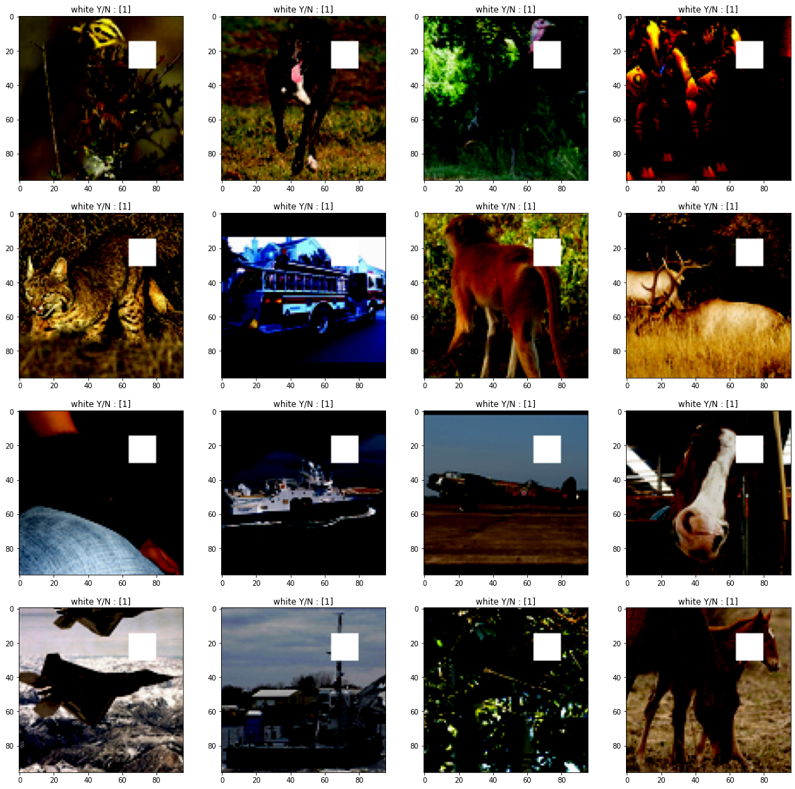
## ( 원문에는 0도있고 1 위치도 다양한데, 내가 한거는 1 위치가 고정되어있다.. 잘못불러온건가? )
그리고나면, 우리는 3가지 클래스를 생성하게 됩니다. 첫번째는 단지 CNN을 사용한 것이고, 두번째는 Multi-Head attention layer를 사용한 것이고, 세번째는 CBAM 모듈을 사용한 것을 의미합니다 .
class ConvPart(nn.Module):
  def __init__(self):
    super().__init__()
    self.cla = nn.Conv2d(3, 32, 5, padding = 2)
    self.p1 = nn.MaxPool2d(2)
    self.c2a = nn.Conv2d(32, 32, 5, padding = 2)
    self.p2 = nn.MaxPool2d(2)
    self.c3 = nn.Conv2d(32, 32, 5, padding = 2)
    self.bn1a = nn.BatchNorm2d(32)
    self.bn2a = nn.BatchNorm2d(32)

  def forward(self, x):
    z = self.bn1a(F.leaky_relu(self.cla(x)))
    z = self.p1(z)
    z = self.bn2a(F.leaky_relu(self.c2a(z)))
    z = self.p2(z)
    z = self.c3(z)
    return z

class Net(nn.Module):
  def __init__(self):
    super().__init__()
    self.conv = ConvPart()
    self.final = nn.Linear(32,1 )
    self.optim = torch.optim.Adam(self.parameters(), lr = 1e-4)

  def forward(self, x):
    z = self.conv(x)
    z = z.mean(3).mean(2)
    p = torch.sigmoid(self.final(z))[:, 0]
    return p, _

class NetMultiheadAttention(nn.Module):
  def __init__(self):
    super().__init__()
    self.conv = ConvPart()
    self.attn1 = MultiheadAttention(n_head = 4, d_model = 32, d_k = 8, d_v = 8)
    self.final = nn.Linear(32, 1)
    self.optim = torch.optim.Adam(self.parameters(), lr = 1e-4)

  def forward(self, x):
    z = self.conv(x)
    q = torch.reshape(z, (z.size(0), -1, z.size(1)))
    q, w = self.attn1(q, q, q)
    q = torch.reshape(q, (z.size(0), z.size(1), z.size(2), z.size(3)))
    z = q.mean(3).mean(2)
    p = torch.sigmoid(self.final(z))[:, 0]
    return p, q

class NetCBAM(nn.Module):
  def __init__(self):
    super().__init__()
    self.conv = ConvPart()
    self.attn1 = CBAM(gate_channels = 32)
    self.final = nn.Linear(32,1)
    self.optim = torch.optim.Adam(self.parameters(), lr = 1e-4)

  def forward(self, x):
    z = self.conv(x)
    q = self.zttn1(z)
    z = q.mean(3).mean(2)
    p = torch.sigmoid(self.final(z))[:, 0]
    return p, q
아래는 학습을 실행하는 코드입니다.
import time
import numpy as np
import torch
import torch.nn as nn
import torch.nn.functional as F
import matplotlib.pyplot as plt
import IPython.display as display

device = 'cuda' if torch.cuda.is_available() else torch.device('cpu')
print(device) # cuda


def plot_without_attention(tr_err, ts_err, tr_acc, ts_acc, img):
  plt.clf()
  fig, axs = plt.subplots(1, 4, figsize = (20, 5))
  axs[0].plot(tr_err, label = 'tr_err')
  axs[0].plot(ts_err, label = 'ts_err')
  axs[0].legend()

  axs[1].plot(tr_acc, label = 'tr_acc')
  axs[1].plot(ts_acc, label = 'ts_acc')
  axs[1].legend()

  axs[2].axis('off')
  axs[3].axis('off')

  display.clear_output(wait = True)
  display.display(plt.gcf())
  time.sleep(0.01)

def plot_with_attention(tr_err, ts_err, tr_acc, ts_acc, img, att_out, no_images = 6):
  plt.clf()
  fig, axs = plt.subplots(1 + no_images, 4, figsize = (20, (no_images + 1) * 5))
  axs[0, 0].plot(tr_err, label = 'tr_err')
  axs[0, 0].plot(ts_err, label = 'ts_err')
  axs[0, 0].legend()

  axs[0, 1].plot(tr_acc, label = 'tr_acc')
  axs[0, 1].plot(ts_acc, label = 'ts_acc')
  axs[0, 1].legend()

  axs[0, 2].axis('off')
  axs[0, 3].axis('off')

  for img_no in range(6):
    im = img[img_no].cpu().detach().numpy().transpose(1,2,0)*0.5 + 0.5
    axs[img_no +1 , 0].imshow(im)
    for i in range(3):
      att_out_img = att_out[img_no, i+1].cpu().detach().numpy()
      axs[img_no + 1, i+1].imshow(att_out_img)
  display.clear_output(wait = True)
  display.display(plt.gcf())
  time.sleep(0.01)

def train(model, att_flag = False, BATCH_SIZE = 32):
  net = model.to(device)
  tr_err, ts_err = [], []
  tr_acc, ts_acc = [], []
  for epoch in range(50):
    errs, accs = [], []
    net.train()
    for i in range(4000//BATCH_SIZE):
      net.optim.zero_grad()
      x, y = getBatch(BATCH_SIZE, i * BATCH_SIZE)
      x = torch.FloatTensor(x).to(device)
      y = torch.FloatTensor(y).to(device)
      p, q = net.forward(x)
      loss = -torch.mean(y*torch.log(p+1e-8) + (1-y)*torch.log(1-p+1e-8))
      loss.backward()
      errs.append(loss.cpu().detach().item())
      pred = torch.round(p)
      accs.append(torch.sum(pred == y).cpu().detach().item()/BATCH_SIZE)
      net.optim.step()

    tr_err.append(np.mean(errs))
    tr_acc.append(np.mean(accs))

    errs, accs = [], []
    net.eval()
    for i in range(1000//BATCH_SIZE):
      x, y = getBatch(BATCH_SIZE, i * BATCH_SIZE + 4000)
      x = torch.FloatTensor(x).to(device)
      y = torch.FloatTensor(y).to(device)
      p, q = net.forward(x)
      loss = -torch.mean(y*torch.log(p+1e-8) + (1-y)*torch.log(1-p+1e-8))
      errs.append(loss.cpu().detach().item())
      pred = torch.round(p)
      accs.append(torch.sum(pred == y).cpu().detach().item()/BATCH_SIZE)
    ts_err.append(np.mean(errs))
    ts_acc.append(np.mean(accs))

    if att_flag == False:
      plot_without_attention(tr_err, ts_err, tr_acc, ts_acc, x[0])
    else:
      plot_with_attention(tr_err, ts_err, tr_acc, ts_acc, x, q)

    print(f'Min train error: {np.min(tr_err)}')
    print(f'Min test error: {np.min(ts_err)}')
CNN 모델의 결과입니다.
- CNN:
model = Net()
train(model, att_flag = False)

>>> Min train error: 1.670841800546441e-06
	Min test error: 4.115260236862043e-05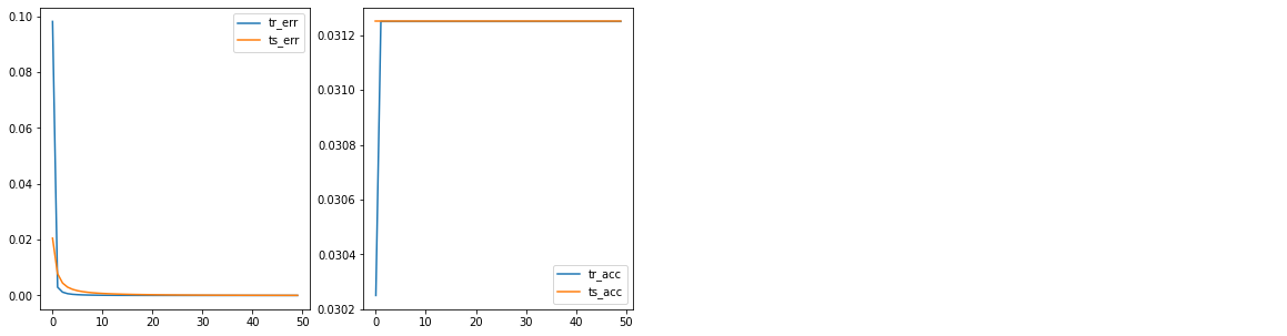
## acc 부분이 왜 일정하게 0.031 이상에서 고정되서 나오는지 모르겠다. 코드 일부 디버깅이 필요하다..
- CNN + Multi-Head attention: attention layer를 추가했을 때, 성능은 향상했지만, 하얀색 패치로 표시된 이미지 부분을 강조하지는 못했습니다.
model = NetMultiheadAttention()
train(model, att_flag=True)
>> Min train error: 0.0012643429860472678
   Min test error: 0.001057574341464187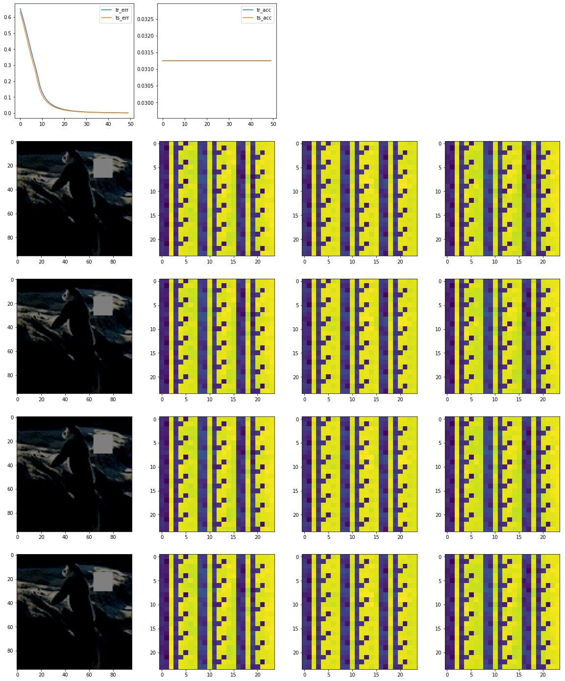
## 왜 사진이 고정되서 나오는지 모르겠다.. for문안에 넣어야할 것 같은데 추후 수정 필요...
'노트 > Python : 프로그래밍' 카테고리의 다른 글
| [python] Colab에서 한글 폰트 사용하기 (0) | 2022.11.01 |
|---|---|
| JVMNotFoundException: No JVM shared library file (libjvm.so) found. Try setting up the JAVA_HOME environment variable properly. (0) | 2022.09.28 |
| [딥러닝 기초] 신경망 코딩하기 (텐서플로우, 파이토치 활용) (0) | 2021.05.19 |
| [시계열] 주가 예측을 위한 RNN/LSTM/GRU 기술적 가이드 (번역) (3) | 2021.03.30 |
| Keras와 OpenCV를 활용하여 웹캠으로 실시간 나이, 성별, 감정 예측 (번역) (3) | 2021.03.26 |