2020. 12. 12. 19:02ㆍ노트/Python : 프로그래밍
원문
towardsdatascience.com/ml-approaches-for-time-series-4d44722e48fe
ML Approaches for Time Series
In this post I play around with some Machine Learning techniques to analyze time series data and explore their potential use in this case…
towardsdatascience.com
ML Approaches for Time Series
비-전통적인 모델로 타임시리즈를 모델링 해봅시다.

이번 포스팅에서는 타임시리즈 데이터를 분석하기위해 머신러닝 기법을 사용하고, 이 시나리오 하에서 잠재적인 사용을 분석할 것입니다.
첫번째 포스트에서는 오직 목차의 첫번째 부분만 발전 시키겠습니다. 나머지는 목차로 부터 분리된 포스트로 접근 가능할 것입니다.
Note : 이번 연구는 2017년 부터 시작되었습니다. 그래서 몇몇 라이브러리들이 업데이트 됬을 수도 있습니다.
목차
1 - 데이터 생성, 창(windows) 과 기초 모델(baseline model)
2 - 유전 프로그래밍 : 기호 회귀 분석(symbolic regression)
3 - 극단의 학습 머신
4 - 가우시안 프로세스
5 - 합성곱 신경망 (CNN)
1 - 데이터 생성, 창(windows) 과 기초 모델(baseline model)
1.1 - 데이터 생성
이번 연구에서는 비주기적 시계열 데이터에 대한 분석을 경험하게 될것입니다. 우리는 3개의 랜덤 변수인 $x_1 , x_2, x_3 $의 합성 데이터를 만들고, 이러한 변수들의 일부 시차들의 선형 조합에 약간의 노이즈를 추가한 반응 변수인 $y$를 결정할 것입니다.
이런 방식으로 우리는 함수가 100% 예측가능하진 않지만, 반응변수가 예측치에 의존한다는 것과, 반응 변수에 대해 이전의 예측치에 대한 시차 (lags)의 효과로 유발된 시간 의존성 (time dependency) 이 있다는 것을 확실히 할 수 있습니다.
이 파이썬 스크립트는 시계열 데이터를 고려하는 창(windows)를 만들 것입니다. 그 이유는 우리가 가능한 가장 완전한 정보를 모델들에게 제공할 수 있게 문제의 틀을 형성하기 위함입니다.
첫번째로 우리가 가진 데이터와 어떤 기술을 우리가 앞으로 적용해야하는지 일단 봅시다.
import numpy as np
import pandas as pd
import matplotlib.pyplot as plt
import copy as cp
N = 600
t = np.arange(0, N, 1).reshape(-1,1)
# 각 숫자에다가 랜덤 오차항을 더함
t = np.array([t[i] + np.random.rand(1)/4 for i in range(len(t)) ])
# 각 숫자에다가 랜덤 오차항을 뺌
t = np.array([t[i] - np.random.rand(1)/7 for i in range(len(t)) ])
t = np.array(np.round(t,2))
x1 = np.round((np.random.random(N) * 5).reshape(-1,1),2)
x2 = np.round((np.random.random(N) * 5).reshape(-1,1),2)
x3 = np.round((np.random.random(N) * 5).reshape(-1,1),2)
n = np.round((np.random.random(N)*2).reshape(-1,1),2)
y = np.array([((np.log(np.abs(2 + x1[t])) - x2[t-1]**2) +
0.02 * x3[t-3]*np.exp(x1[t-1])) for t in range(len(t))])
y = np.round(y+n ,2 )fig, (ax1,ax2) = plt.subplots(nrows=2)
fig.set_size_inches(30,14)
ax1.plot(y, marker = "o") # 600일간 데이터
ax2.plot(y[:100], marker = "o") # 100일간 데이터
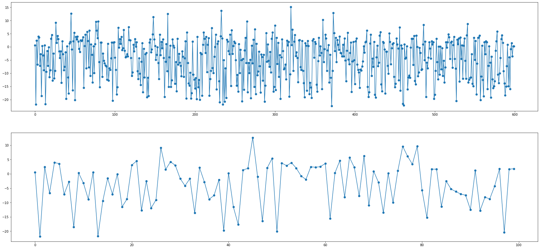
이제, 우리는 3개의 독립변수에 노이즈를 첨가한 반응변수 y 함수를 가지고 있습니다.
또한 반응 변수는 직접적으로 주어진 지점에서 그들의 값 뿐만 아니라 독립 변수의 시차에 연관 (correlated) 되어 있습니다. 이 방식대로 우리는 시간 의존성을 보장하고, 우리의 모델이 이런 행동들을 식별하도록 만들 것입니다.
또한, 타임스템프의 간격이 균일하지 않습니다. 이런 식으로, 우리는 우리의 모델들이 단지 관측 수 (행)로 시리즈를 다룰 수 없기 때문에 시간 의존성을 이해하기 원한다는 생각을 굳건히 합니다.
우리는 데이터에 높은 비 선형성을 유도할 목적으로 지수연산자와 로그연산자를 포함시켰습니다.
1.2 - 창(Windows) 형성하기
이번 연구에서 모든 모델들이 따르는 접근은 정확한 예측을 달성하기 위해 우리가 가지고 있는 정보를 과거로 부터 주어진 시점에서 가능한 가장 완전한 정보를 모델에 제공하는 고정된 창(windows) 으로 재구성하는 것입니다. 추가적으로, 우리는 반응 변수 자체의 이전 값을 독립 변수로 제공하는 것이 모형에 어떤 영향을 미치는지 확인할 것입니다.
어떻게 되는지 한번 봅시다.
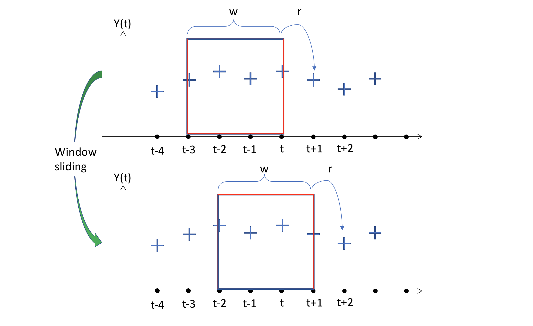
이 그림은 오직 시간 축과 반응변수만을 보여줍니다. 우리의 경우, t 값에 대한 반응 변수들은 3개 의 변수들이 있다는 것을 기억하세요.
제일 위에있는 그림은 w 크기로 선택된 (그리고 고정된) 창을 볼 수 있습니다. 이 경우에는 창의 크기가 4 이구요. 이것은 모델이 t+1 지점에서의 예측을 통해 창에 포함된 정보를 매핑한다는 사실을 의미합니다. 반응의 크기는 r 이 있는데, 우리는 과거에 몇가지 타임 스텝을 예측할 수 있었기 때문입니다. 이는 many-to-many 관계를 가집니다. 단순하고 쉬운 시각화를 위해서, 우리는 r=1 로 두겠습니다.
우리는 이제 Sliding Window 의 효과를 확인할 수 있습니다. 모델이 매핑함수를 찾기위해 갖게되는 input과 output의 다음 짝은 window를 한 스텝 미래로 움직음으로써 얻어집니다. 그리고 이전의 스텝에서 했던 것 처럼 같은 동작을 이어나갑니다.
Ok. 그러면, 어떻게 우리가 현재 데이터 셋에 이것을 적용할 수 있을까요? 우리가 필요한 것을 한번 봅시다. 그리고 우리의 유용한 함수를 만들어봅시다.
하지만 첫번째로, 우리는 시간이 절대값이 되는 것을 원하지 않습니다. 관찰 사이의 경과시간이 어느것인지 아는 것이 더 흥미로운 점입니다. (데이터가 균일하지 않다는 것을 기억하세요!). 그래서, $\Delta t$를 만들고, 우리의 데이터에 적용해봅시다.
dataset = pd.DataFrame(np.concatenate((t,x1,x2,x3,y), axis=1),
                       columns = ['t','x1','x2','x30','y'])
dataset[:7]
deltaT = np.array([(dataset.t[i+1] - dataset.t[i]) for i in range(len(dataset)-1)])
deltaT = np.concatenate( (np.array([0]), deltaT))
deltaT[:7]
dataset.insert(1,'∆t',deltaT)
dataset.head(3)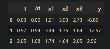
이제 우리의 데이터셋이 어떻게 생겼는지 알게되었습니다. 우리의 helper 함수가 테이블의 구성으로 무엇을 하기 원하는지 재현해봅시다.
window사이즈가 4인 경우에 :
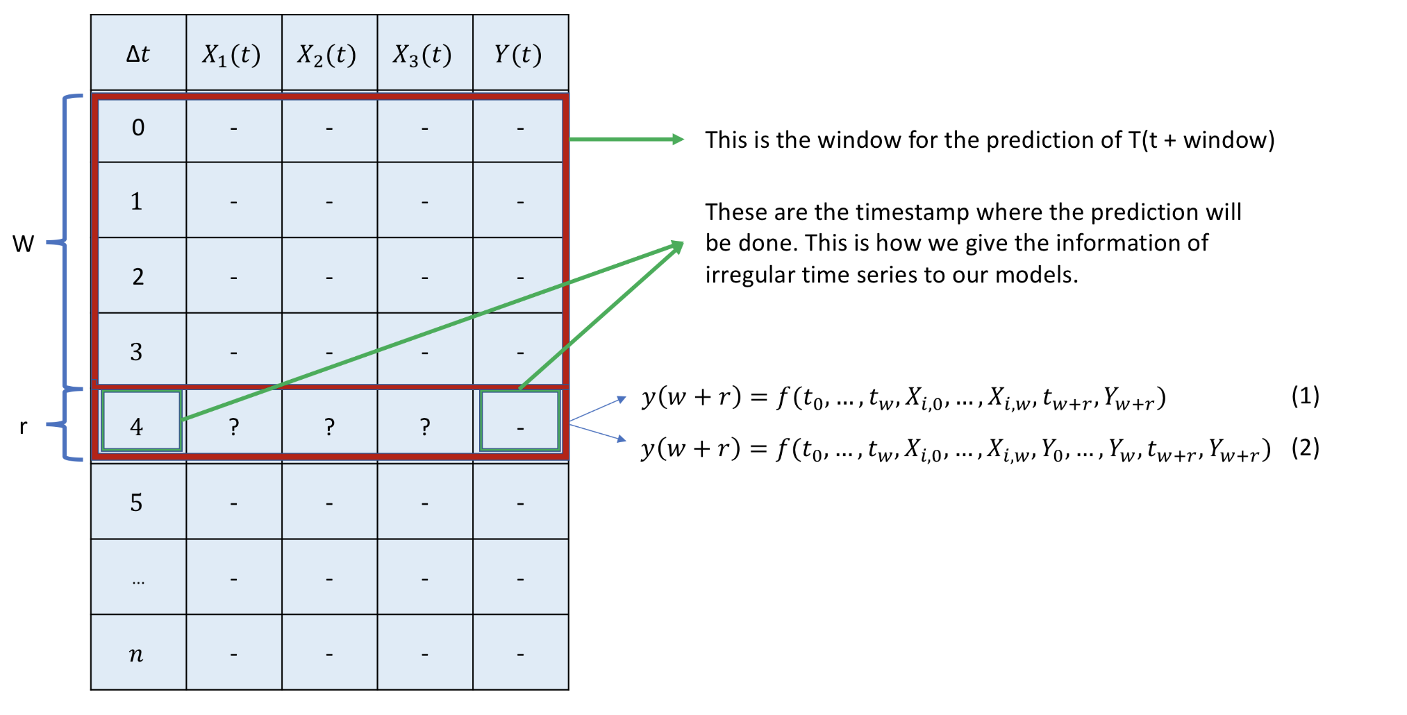
우리의 함수가 하는 것은 window 안에 포함되어있는 모든 정보를 압축 (flatten) 하는 것입니다. 이 정보는 W window 내의 모든 값이며, 예측을 원하는 시간의 타임스탬프를 뜻합니다.
이 방식으로, 우리는 시스템을 모델링 하기 위한 2가지 다른 등식을 가지고 있으며, 새로운 예측치로 반응변 수의 이전의 값을 포함하고 있는 지에 따라 의존합니다.
함수가 리턴해야하는 결과는 이렇게 생겼습니다 :
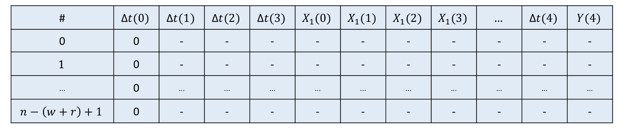
우리는 $ l = n - (w+r) +1 $개의 windows를 만들 수 있을 것입니다, 왜냐하면 $Y(0)$ 의 첫번째 값에 대한 이전 정보가 없기 때문에 첫번째 행이 손실되기 때문입니다.
우리가 언급해온 모든 시차들은 모델의 새로운 예측치로 행동합니다 ( 이 시각화에서 Y의 이전 값이 포함되지 않았지만, 같은 값을 $X_i$ 로 따르게될 것입니다. ) 그리고 나서, (경과한) 타임스탬프는 여기서 우리가 원하는 예측값이 ∆t(4)가 되길 원할 것이며, 그에 따르는 예측에 대한 값이 Y(4)가 되야합니다. 모든 첫번째 ∆t(0) 가 0으로 초기화된다는 점에 주목하세요. 모든 window를 같은 범위로 표준화 하기를 원하기 때문입니다.
여기에 이 과정을 달성할 수 있는 코드를 만들었습니다. WindowSlider 형태의 함수가 있고 , 이 함수로 부터 파라미터를 변화하면서 다른 windows를 구성하는 객체를 만들 수 있습니다.
class WindowSlider(object):
    def __init__(self, window_size = 5):
        """
        Window Slider object
        ====================
        w: window_size - number of time steps to look back
        o: offset between last reading and temperature
        r: response_size - number of time steps to predict
        l: maximum length to slide - (#obeservation - w)
        p: final predictors - (# predictors *w)
        """
        self.w = window_size
        self.o = 0
        self.r = 1
        self.l = 0
        self.p = 0
        self.names = []

    def re_init(self, arr):
        """
        Helper function to initializate to 0 a vector
        """
        arr = np.cumsum(arr)
        return arr - arr[0]

    def collect_windows(self, X, window_size = 5, offset = 0, previous_y = False):
        """
        Input: X is the input matrix, each column is a variable
        Returns : different mappings window-output
        """
        cols = len(list(X))-1
        N = len(X)

        self.o = offset
        self.w = window_size
        self.l = N - (self.w + self.r) + 1
        if not previous_y:
            self.p = cols * self.w
        if previous_y:
            self.p = (cols +1) * self.w

        # Create the names of the variables in the window
        # Check first if we need to create that for the response itself
        if previous_y:
            x = cp.deepcopy(X)
        if not previous_y:
            x = X.drop(X.columns[-1], axis=1)

        for j , col in enumerate(list(x)):
            for i in range(self.w):
                name = col + ("(%d)" % (i+1))
                self.names.append(name)

        # Incorporate the timestampes where we want to predict
        for k in range(self.r):
            name = "∆t" + ("(%d)" % (self.w + k +1))
            self.names.append(name)

        self.names.append("Y")

        df = pd.DataFrame(np.zeros(shape = (self.l, (self.p + self.r +1))),
                         columns = self.names)

        # Populate by rows in the new dataframe
        for i in range(self.l):
            slices = np.array([])

            # Flatten the lags of predictors
            for p in range(x.shape[1]):
                line = X.values[i:self.w+i,p]
                # Reinitialization at every window for ∆T
                if p == 0:
                    line = self.re_init(line)

                # Concatenate the lines in one slice
                slices = np.concatenate((slices,line))

            # Incorporate the timestamps where we want to predict
            line = np.array([self.re_init(X.values[i:i+self.w +self.r,0])[-1]])
            y = np.array(X.values[self.w + i + self.r -1, -1]).reshape(1,)
            slices = np.concatenate((slices,line,y))

            # Incorporate the slice to the cake (df)
            df.iloc[i,:] = slices

        return df
1.2 - 기본 모델 (Baseline Model)
"항상 단순한 것을 먼저해라. 필요한 경우에만 지능을 적용해라" - Thad Starner
Windows 생성
w = 5

train_constructor = WindowSlider()
train_windows = train_constructor.collect_windows(trainset.iloc[:,1:],
                                                 previous_y = False)

test_constructor = WindowSlider()
test_windows = test_constructor.collect_windows(testset.iloc[:,1:],
                                                 previous_y = False)

train_constructor_y_inc = WindowSlider()
train_windows_y_inc = train_constructor_y_inc.collect_windows(trainset.iloc[:,1:],
                                                             previous_y = True)

test_constructor_y_inc = WindowSlider()
test_windows_y_inc = test_constructor_y_inc.collect_windows(testset.iloc[:,1:],
                                                             previous_y = True)

train_windows.head(3)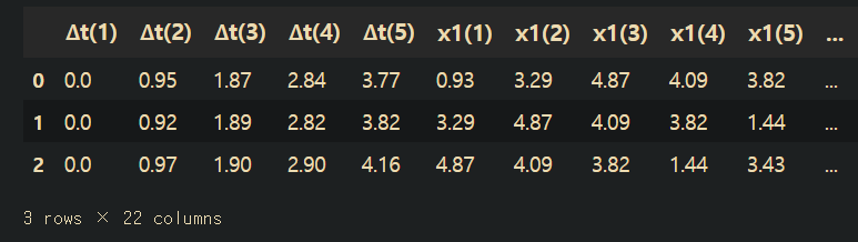
이제 모든 예측치, 남은 변수들의 과거 타임 스텝의 기록(window_length) 과 ∆t 의 누적 합을 어떻게 windows가 가져오는지 볼 수 있습니다.
예측치(prediction) = 현재(current)
우선 다음 타임스탬프의 예측으로 마지막 값(각 예측 지점에서 현재 값)을 주는 간단한 모델부터 시작해보겠습니다.
# ________________ Y_pred = current Y ________________

bl_trainset = cp.deepcopy(trainset)
bl_testset = cp.deepcopy(testset)

bl_train_y = pd.DataFrame(bl_trainset['y'])
bl_train_y_pred = bl_train_y.shift(periods = 1)

bl_y = pd.DataFrame(bl_testset['y'])
bl_y_pred = bl_y.shift(periods = 1)

bl_residuals = bl_y_pred - bl_y
bl_rmse = np.sqrt(np.sum(np.power(bl_residuals,2)) / len(bl_residuals))
print("RMSE = %.2f" % bl_rmse)
print("Time to train  = 0 secconds")

>>> RMSE = 9.78
   Time to train  = 0 secconds
fig, ax1 = plt.subplots(nrows=1)
fig.set_size_inches(40,10)
ax1.plot(bl_y, marker = "o" , label = "actual") # 100일간 데이터
ax1.plot(bl_y_pred, marker = "o", label = "predict") # 100일간 데이터
ax1.legend(prop={'size':30})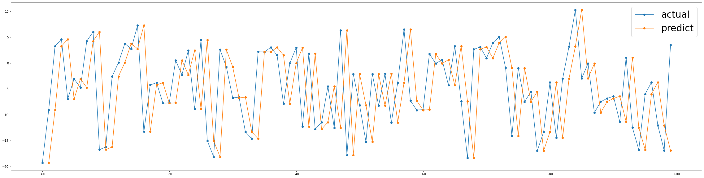
결론 우리는 이미 다가오는 결과를 비교할 가치가 있습니다.
우리는 주어진 현재 값을 예측 값으로 고려하는 단순한 룰을 적용해보았습니다. 시계열에서 반응 변수의 값이 더욱 안정적이라면(stable) (a.k.a stationary) , 이 방식은 때때로 ML 알고리즘보다 놀랍게도 더 나은 성능을 보여줄 것입니다. 이런 경우에 데이터의 지그재그(zig-zag)는 악명이 높아 예측력이 떨어지는 것으로 이어집니다.
다중 선형 회귀 (Multiple Linear Regression)
우리의 다음접근은 다중 선형회귀 모델을 구성하는 것입니다.
# ______________ MULTIPLE LINEAR REGRESSION ______________ #

import sklearn
from sklearn.linear_model import LinearRegression
import time
lr_model = LinearRegression()
lr_model.fit(trainset.iloc[:,:-1], trainset.iloc[:,-1])

t0 = time.time()
lr_y = testset["y"].values
lr_y_fit = lr_model.predict(trainset.iloc[:,:-1])
lr_y_pred = lr_model.predict(testset.iloc[:,:-1])
tF = time.time()

lr_residuals = lr_y_pred - lr_y
lr_rmse = np.sqrt(np.sum(np.power(lr_residuals,2))/len(lr_residuals))
print("RMSE = %.2f" % lr_rmse)
print("Time to train = %.2f seconds" % (tF-t0))

>>> RMSE = 7.52
  Time to train = 0.01 seconds
fig, ax1 = plt.subplots(nrows=1)
fig.set_size_inches(40,10)
ax1.plot(lr_y, marker = "o" , label = "actual") # 100일간 데이터
ax1.plot(lr_y_pred, marker = "o", label = "predict") # 100일간 데이터
ax1.legend(prop={'size':30})
결론 다중 선형 회귀 모형이 얼마나 반응 변수의 동작을 포착하지 못하는지 알 수 있습니다. 이는, 반응변수와 독립변수 간의 비- 선형 관계 때문인데요. 또한 주어진 시간에 반응변수에게 영향을 미치는 것은 변수들간의 시차입니다. 따라서 이 관계를 매핑할 수 없는 모형에 대해 서로 다른 행에 값(values)들이 있습니다.
나는(저자는) windows의 구조에 대해 설명할 때 우리가 만든 가정을 이제 어떻게 확인해야 할지 궁금해졌습니다. 우리는 모든 예측 지점에 대해 완전한 정보 셋을 구성하기 원한다고 말해보겠습니다. 그래서, windows를 구성한 후의 예측력이 올라갸아합니다... 한번 가보죠 !
Windows를 가진 다중 선형 회귀 ( MLR with the Windows)
# ___________ MULTIPLE LINEAR REGRESSION ON WINDOWS ___________
lr_model = LinearRegression()
lr_model.fit(train_windows.iloc[:,:-1], train_windows.iloc[:,-1])

t0 = time.time()
lr_y = test_windows['Y'].values
lr_y_fit = lr_model.predict(train_windows.iloc[:,:-1])
lr_y_pred = lr_model.predict(test_windows.iloc[:,:-1])
tF = time.time()

lr_residuals = lr_y_pred - lr_y
lr_rmse = np.sqrt(np.sum(np.power(lr_residuals,2))/ len(lr_residuals))
print("RMSE = %.2f" %lr_rmse)
print("Time to Train = %.2f seconds" % (tF-t0))
>>> RMSE = 2.51
   Time to Train = 0.01 seconds
fig, ax1 = plt.subplots(nrows=1)
fig.set_size_inches(40,10)
ax1.plot(lr_y, marker = "o" , label = "actual") # 100일간 데이터
ax1.plot(lr_y_pred, marker = "o" , label = "predict") # 100일간 데이터
ax1.legend(prop={'size':30})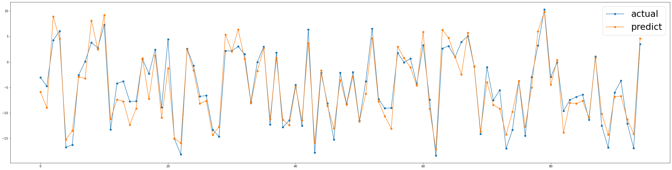
Wow! 굉장한 향상을 보였습니다.
이제 우리는 물리칠 수 있는 매우 강력한 모델이 있습니다. 새로운 windows 로, 모델은 전체 window 정보와 반응변수간의 관계를 찾을 수 있을 것으로 보입니다.
2 — 기호 회귀분석 (Symbolic Regression)
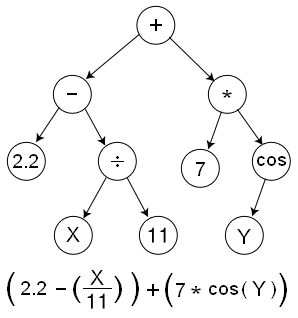
기호 회귀분석은 주어진 데이터셋을 적합하는 최적의 모델을 찾기위한 수학적 표현의 공간을 찾는 회귀 분석의 한 유형입니다.
기호 회귀분석의 기본은 유전 프로그래밍인데요, 그래서 진화 알고리즘 (a.k.a. 유전 알고리즘 (Genetic Algorithm - GA)이라고 합니다.
어떻게 알고리즘이 작동하는지 몇마디로 요약하면, 첫번째로 위의 그림과 같이, 수학적 표현이 트리 구조로 표현된다는 것을 이해할 필요가 있습니다.
이런 방식으로 알고리즘은 1세대에서 많은 나무의 개체수를 가지고 시작할 것이며, 이는 적합 함수 (fitness fuction)에 따라 측정될 것입니다. 우리의 경우에는 RMSE이죠. 각 세대에 가장 우수한 개인들은 그들 사이를 가로지르고 탐험과 무작위성을 포함하기 위해 일부 돌연변이를 적용합니다. 이 반복적인 알고리즘은 정지 조건이 충족될 때 끝납니다.
이 비디오는 유전 프로그래밍에 대한 훌륭한 설명을 해주고 있습니다.
모델
#######################
# CREATION OF THE MODEL
#######################

# !pip instal gplearn
import gplearn as gpl
from gplearn.genetic import SymbolicRegressor

# It is possible to create custom operations to be considered in the tree
def _xexp(x):
    a = np.exp(x);
    a[np.abs(a) > 1e+9] = 1e+9
    return a

xexp = gpl.functions.make_function( function = _xexp , name = 'xexp', arity=1)
#function_set = ['add', 'sub','mul','div','sin','log'] # ,xexp]
function_set = ['add', 'sub','mul','div']

if 'model' in locals(): del model
model = SymbolicRegressor(population_size = 3000,
                         tournament_size = 5,
                         generations = 25,
                         stopping_criteria = 0.1,
                         function_set = function_set,
                         metric = 'rmse',
                         p_crossover = 0.65,
                         p_subtree_mutation = 0.15,
                         p_hoist_mutation = 0.05,
                         p_point_mutation = 0.1,
                         verbose = 1,
                         random_state = None,
                         n_jobs = -1)

###########################################################
# TRAIN THE NETWORK AND PREDICT - Without previous values y
###########################################################

# Train
t0 = time.time()
model.fit(train_windows.values[:,:-1], train_windows.values[:,-1])
tF = time.time()

# Predict
sr_y_fit = model.predict(train_windows.values[:,:-1]).reshape(-1,1)
sr_y_pred = model.predict(test_windows.values[:,:-1]).reshape(-1,1)

# Calculating Errors
sr_residuals = sr_y_pred - testset.iloc[5:,-1].values.reshape(-1,1)
sr_rmse = np.sqrt(np.sum(np.power(sr_residuals,2))/ len(sr_residuals))
print("RMSE = %f" % sr_rmse)
print("Time to train %.2f" % (tF-t0))
print(model._program)
fig, ax1  = plt.subplots(nrows=1)
fig.set_size_inches(40,10)


ax1.plot(testset.iloc[5:,-1].values, marker = "o", label="actual") # 100일간 데이터
ax1.plot(sr_y_pred, marker = "o", label="predict") # 100일간 데이터
ax1.legend(prop={'size':30})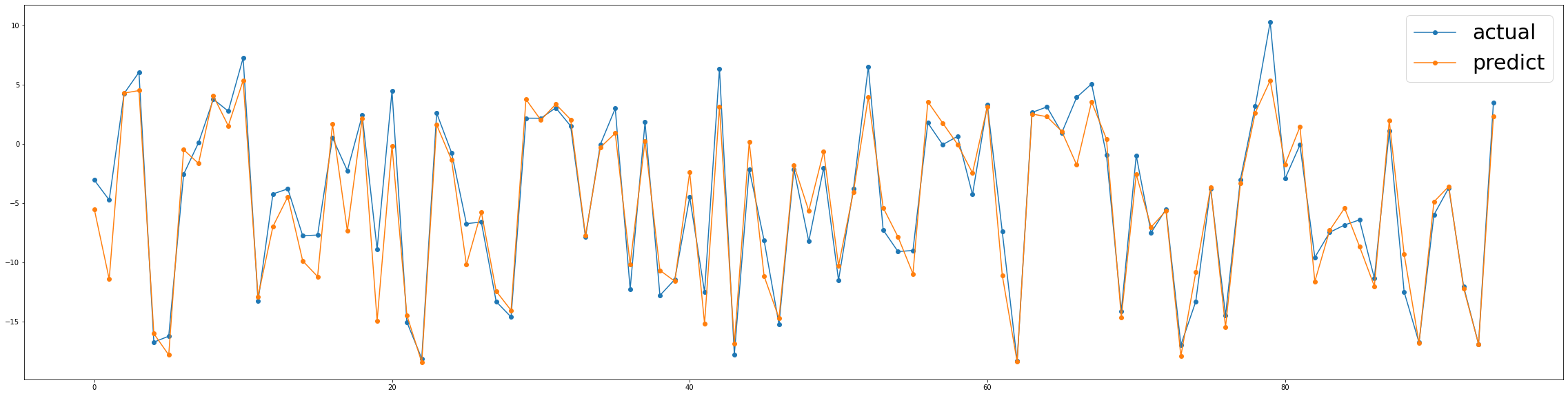
결론
우리는 상징적 회귀분석이 검증데이터에 거의 완벽한 적합과 함께 상당히 좋은 성능을 발휘한다는 것을 보고 있습니다.
놀랍게도, 나는 더 많은 훈련 시간의 단점을 가지고도 가장 단순한 네개의 operators (덧셈, 뺄셈, 곱셈, 나눗셈) 만 포함시킴으로써 최고의 정확도를 달성했습니다.
나는 당신이 모델의 다른 파라미터들을 시도해보고 결과를 향상시키기를 기대합니다!
3 — 극단의 학습 머신 (Extreme Learning Machines)

극단의 학습 머신은 중요하고 알려진 머신러닝 기법입니다. 이 기법의 주요 측면은 모델의 파라미터들을 계산하기위해 학습 과정을 필요로 하지 않는다는 점입니다.
본질적으로, 한 EML 은 단층 피드포워드 신경망(Single-Layer-Feed-Forward Neural Network) 입니다 (SLFN) ELM 이론은 히든 레이어의 가중치 값이 조정될 필요가 없으며, 따라서 트레이닝 데이터와 독립적일 필요가 있다는 것을 보여줍니다.
보편적인 근사이론 (universal approximation property) 은 EML이 모든 숨겨진 뉴런에 대한 파라미터를 학습하기에 충분한 데이터를 가지고 있다면, 원하는 정확도로 회귀 문제를 해결할 수 있다는 것을 의미합니다.
EML은 또한 모델 구조와 정규화(regularization)의 이점을 얻는데, 이는 무작위 초기화 및 오버피팅의 부정적인 효과를 감소시킨다는 것입니다.
N개의 트레이닝 샘플 (x, t) 를 고려해보면, L개의 히든 신경망 출력값을 가진 SLFN은 다음과 같습니다 :

네트워크의 target, inputs , outputs 의 관계는 다음과 같습니다 :

히든 신경망이 입력 데이터를 두단계에 걸쳐 다른 표현으로 변형시킵니다. 첫번째로, 데이터는 입력층의 가중치와 편향을 통해 히든 레이어에 투영된 다음, 비선형 활성화 함수의 결과에 적용됩니다.
실제로, ELMs은 행렬 형태로 공통 신경망으로 해결됩니다. 행렬 형태는 다음과 같이 표현됩니다. :
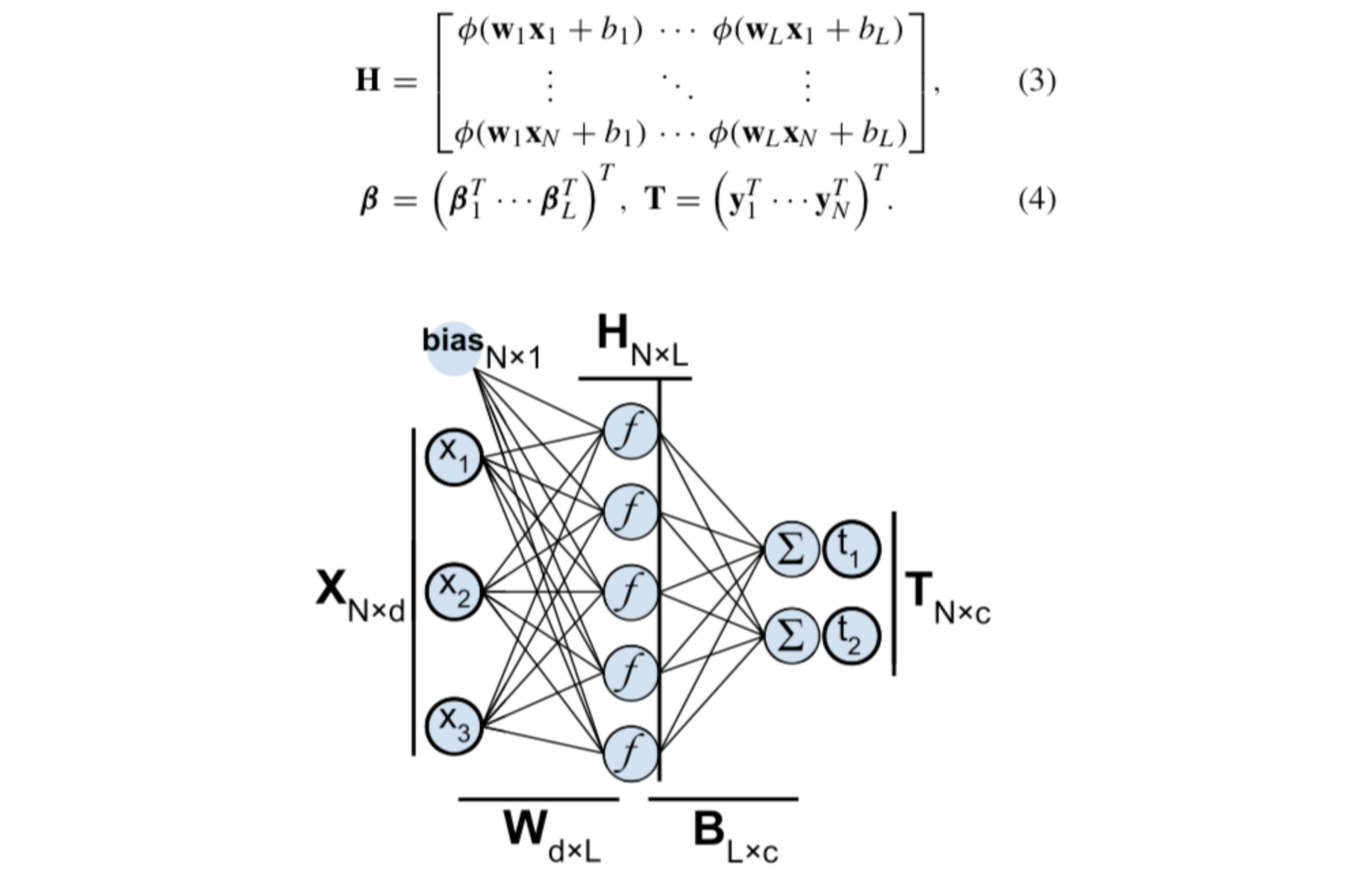
그리고 여기에 이 방법이 도출하는 중요한 부분이 있습니다. T가 우리가 도달하고자 하는 target임을 감안할 때, 최소 제곱 오차 항이 있는 시스템은 무어-펜로즈 일반화된 유사 역행렬 (Moore-Penrose generalized inverse) 을 사용한 독특한 솔루션을 사용할 수 있습니다. 따라서, 우리는 한번의 작업으로 target T를 예측할 수 있는 최소한의 오차를 가진 해결책이 되는 히든레이어의 가중치 값을 계산할 수 있습니다.

이 가짜역행렬(presudoinverse)은 단수값 분해(Singular Value Decomposition)를 사용하여 계산되었습니다.
이 글에서는 어떻게 EML이 작동하는지, 그리고 EML의 높은 성능의 Toolbox 패키지와 MATLAB과 Python의 실행에 대해 상세하게 잘 정리된 설명이 있습니다.
모델
class Network(object):
    def __init__(self, input_dim, hidden_dim = 10, output_dim = 1):
        """
        Neural Network object
        """
        self.N = input_dim
        self.M = hidden_dim
        self.O = output_dim

        self.W1 = np.matrix(np.random.rand(self.N, self.M))
        self.W2 = np.matrix(np.random.rand(self.M, self.O))

        self.U = 0
        self.V = 0
        self.S = 0
        self.H = 0
        self.alpha = 0 # for regularization

    # Helper function
    def sigmoid(self, x):
        return 1.0 / (1.0 + np.exp(-0.1 * x)) - 0.5

    def predict(self,x):
        """
        Forward pass to calculate the output
        """
        x = np.matrix(x)
        y = self.sigmoid( x @ self.W1) @ self.W2
        return y

    def train(self, x, y):
        """
        Compute W2 that lead to minimal LS
        """
        X = np.matrix(x)
        Y = np.matrix(y)
        self.H = np.matrix(self.sigmoid(X @ self.W1))
        H = cp.deepcopy(self.H)

        self.svd(H)
        iH = np.matrix(self.V) @ np.matrix(np.diag(self.S)).I @ np.matrix(self.U).T

        self.W2 = iH * Y
        print('W2 values updated...')
        return H @ self.W2 - Y

    def svd(self, h):
        """
        Compute the Singualr Value Decomposition of a matrix H
        """
        H = np.matrix(h)
        self.U , self.S , Vt = np.linalg.svd(H, full_matrices = False)
        self.V = np.matrix(Vt).T
        print('SVD computed.. calulating Pseudoinverse..')
        return np.matrix(self.U), np.matrix(self.S), np.matrix(self.V)
y의 이전 값을 features로 고려하지 않겠습니다.
###############################################################
# TRAIN THE NETWORK AND PREDICT - Without previous values of y
###############################################################

in_dim = train_windows.shape[1] -1
NN = Network(input_dim = in_dim, hidden_dim = 20, output_dim = 1)
t0 = time.time()
eml_residuals = NN.train(x =train_windows.iloc[:,:-1],
                        y = train_windows.iloc[:,-1].values.reshape(-1,1))
tF = time.time()

fit = NN.predict(train_windows.iloc[:,:-1])
predictions = NN.predict(test_windows.iloc[:,:-1])

eml_fit = cp.deepcopy(fit)
eml_pred = cp.deepcopy(predictions)

eml_residuals = eml_pred - testset.iloc[w:,-1].values.reshape(-1,1)
eml_rmse = np.sqrt(np.sum(np.power(eml_residuals,2)) / len(eml_residuals))
print('RMSE = %.2f' % eml_rmse)
print("Time to train %.2f" % ( tF-t0))

>>>  ###############################################################
# TRAIN THE NETWORK AND PREDICT - Without previous values of y
###############################################################

in_dim = train_windows.shape[1] -1
NN = Network(input_dim = in_dim, hidden_dim = 20, output_dim = 1)
t0 = time.time()
eml_residuals = NN.train(x =train_windows.iloc[:,:-1],
                        y = train_windows.iloc[:,-1].values.reshape(-1,1))
tF = time.time()

fit = NN.predict(train_windows.iloc[:,:-1])
predictions = NN.predict(test_windows.iloc[:,:-1])

eml_fit = cp.deepcopy(fit)
eml_pred = cp.deepcopy(predictions)

eml_residuals = eml_pred - testset.iloc[w:,-1].values.reshape(-1,1)
eml_rmse = np.sqrt(np.sum(np.power(eml_residuals,2)) / len(eml_residuals))
print('RMSE = %.2f' % eml_rmse)
print("Time to train %.2f" % ( tF-t0))

>>> SVD computed.. calulating Pseudoinverse..
    W2 values updated...
    RMSE = 3.70
    Time to train 0.03
fig, ax1 = plt.subplots(nrows=1)
fig.set_size_inches(40,10)
ax1.plot(testset.iloc[w:,-1].values, marker = "o", label = "actual") # 100일간 데이터
ax1.plot(eml_pred, marker = "o", label="predict") # 100일간 데이터
ax1.legend(prop={'size':30})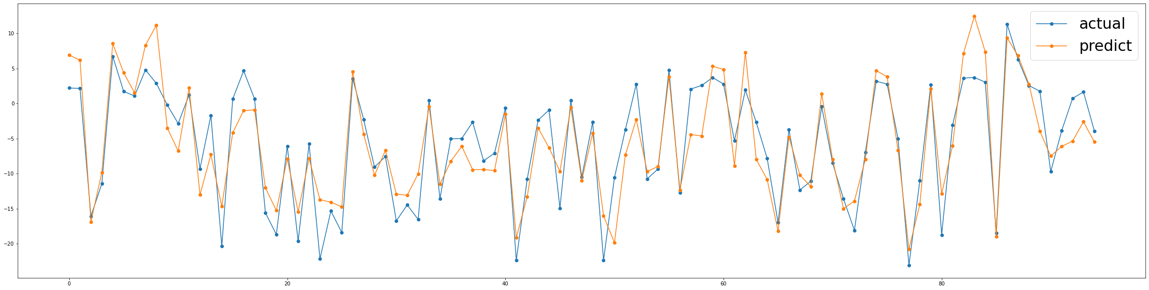
결론
우리는 어떻게 EMLs가 우리의 데이터에 굉장한 예측력을 가지는지 볼 수 있었습니다. 또한, 반응변수의 이전 값을 예측 변수로 포함시킨 결과도 훨씬 더 나빠졌습니다.
확실히, EMLs는 계속해서 탐구해야할 모델입니다. 이것은 빠르게 구현함으로써 이미 그들의 엄청난 힘을 보여주었고, 단순한 역행렬과 몇번의 조작으로 그 정확성(accuracy)을 계산할 수 있었습니다.
온라인 학습
EMLs의 절대적으로 큰 장점은 온라인 모델을 구현하기 위해 계산적으로 매우 저렴하다는 것입니다. 이 글에서는 업데이트 및 다운데이트 작업에 대한 자세한 정보를 볼 수 있습니다.
몇줄 안가서, 우리는 모델이 적응이되었다고 말할 수 있으며, 만약 예측 오차가 안정된 임계값을 초과하면, 이 특정한 데이터 지점이 SVD에 통합됩니다. 그래서 모델이 값비싼 완전한 재트레이닝을 요구하지 않습니다. 이런 방식으로 모델은 프로세스에서 일어날 수 있는 변화로 부터 적응하고 배울 수 있습니다.
4 — Gaussian Processes
가우시안 프로세스 (Gaussian Processes) 는 그러한 변수의 모든 유한한 집합이 다변량 정규 분포를 가지도록 하는 랜덤 변수의 집합이며, 이는 이들 변수의 가능한 모든 선형 조합이 정규 분포를 따른 다는 것을 의미합니다. (가우시안 프로세스는 다변량 정규 분포의 유한-차원의 일반화로 볼 수 있습니다)
GP의 분포는 모든 랜덤 변수들의 결합 분포입니다. 몇마디로 줄이자면, GPs는 보이지 않는 지점에 대한 값을 예측하는 점들 사이의 유사성을 결정하는 커널 함수를 사용합니다.
이 비디오는 CO2 수준을 예측하는 가우시안 프로세스에 대한 훌륭하고 짧은 인트로를 소개합니다.
이 책은 가우시안 프로세스에 대한 주요 가이드 입니다.
GP의 한가지 분명한 장점은 예측을 중심으로 신뢰 구간을 쉽게 형성하기에, 모든 예측치에서 표준 편차를 얻을 수 있다는 사실입니다.
모델
매우 간단한 CNN을 가져와 보겠습니다 :
#######################
# CREATION OF THE MODEL
#######################

from sklearn.gaussian_process import GaussianProcessRegressor as GP
from sklearn.gaussian_process.kernels import ConstantKernel as C
from sklearn.gaussian_process.kernels import RBF
from sklearn.gaussian_process.kernels import ExpSineSquared as ES
from sklearn.gaussian_process.kernels import DotProduct as DP
from sklearn.gaussian_process.kernels import Matern
from sklearn.gaussian_process.kernels import WhiteKernel as WK

l = 2.
kernels = {'cnt': C(constant_value=0.1),
          'rbf': RBF(length_scale=1),
          'ex2': ES(length_scale=1),
          'dot': DP(sigma_0 = 0.1),
          'mat': Matern(length_scale=1, nu=1.5),
          'whi': WK(noise_level=0.01)}
k = kernels['cnt'] + kernels['ex2'] + kernels['rbf']
if 'gp' in locals():
    del gp
gp = GP(kernel = k , n_restarts_optimizer = 9, normalize_y = True)
y의 이전값을 feature로 고려하지 않겠습니다.
#####################################################
# TRAIN THE NETWORK AND PREDICT - Without previous y
#####################################################

# Train
tranX = train_windows.values[:,:-1]
tranY = train_windows.values[:,-1]
testX = test_windows.values[:,:-1]
testY = test_windows.values[:,-1]

t0 = time.time()
gp.fit(train_windows.values[:,:-1], train_windows.values[:,-1])
tF = time.time()

# Predict
gp_y_fit = gp.predict(train_windows.values[:,:-1], return_std = False)
gp_y_pred, gp_y_std = gp.predict(test_windows.iloc[:,:-1], return_std = True)

gp_y_up = (gp_y_pred + 1.96 * gp_y_std).reshape(-1,)
gp_y_lw = (gp_y_pred - 1.96 * gp_y_std).reshape(-1,)
gp_y_pred = gp_y_pred.reshape(-1,1)

# Calculating Errors
gp_residuals = gp_y_pred - testset.iloc[5:,-1].values.reshape(-1,1)
gp_rmse = np.sqrt(np.sum(np.power(gp_residuals,2))/ len(gp_residuals))
print("RMSE = %f" % gp_rmse)
print("Time to train % .2f" %(tF-t0))

>>> RMSE = 1.429122
    Time to train  22.79
fig, ax1 = plt.subplots(nrows=1)
fig.set_size_inches(40,10)
ax1.plot(testset.iloc[5:,-1].values, marker = "o", label = "actual") # 100일간 데이터
ax1.plot(gp_y_pred, marker = "o", label="predict") # 100일간 데이터
ax1.legend(prop={'size':30})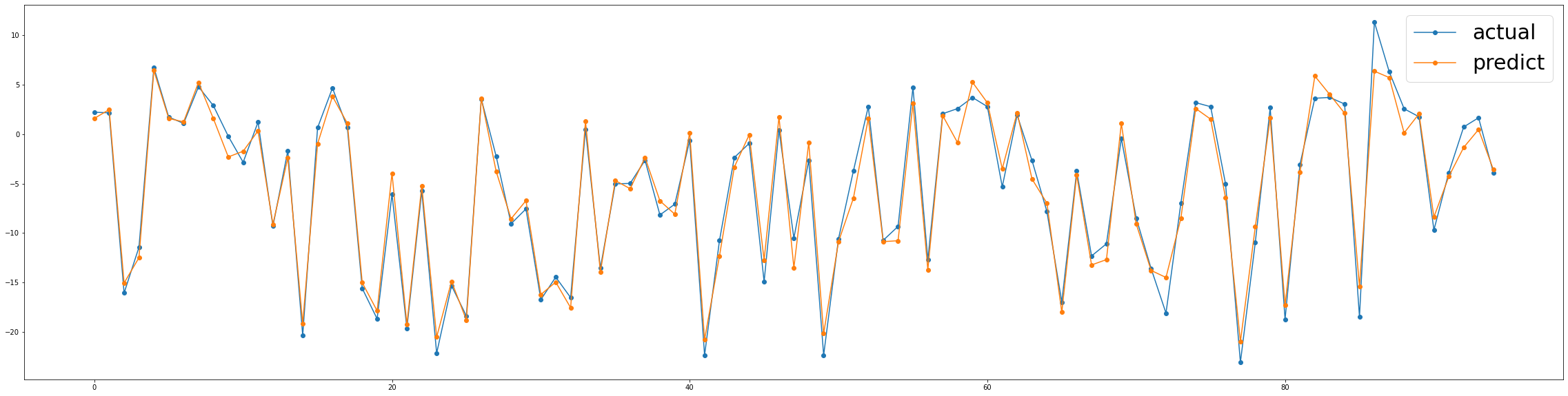
결론
우리는 가우시안 프로세스가 또 다른 높은 예측력을 가진 얼마나 아름다운 접근인지 볼 수 있었습니다. 이 모델은 또한 반응 변수의 이전 값을 예측치로 가져왔을 때 결과가 더욱 나빠졌습니다.
요점은, 튜닝된 커널의 거의 무한한 조합을 가지고 놀 수 있다는 것입니다. 즉, 그들의 결합 분포가 우리의 모델에 더 잘 맞는 랜덤 변수의 조합을 찾을 수 있다는 것입니다. 나는 당신만의 커널을 시도해보고, 이 결과를 향상시키길 권합니다.
5 — Convolutional NN
아이디어는 주어진 시간에 프로세스의 상태를 이전의 값의 window가 pucture로 정의한다는 것입니다.
그래서, 우리는 "pictures"를 반응 변수에 매핑하는 패턴을 찾고자 하기 때문에 이미지 인식의 평행도 (parallelism)을 사용하고자 합니다. 우리는 우리의 timeseries.py에 새로운 함수인 WindowsToPictures()를 포함하였습니다.
이 함수는 우리가 inputs 값으로 사용하던 windows를 가져가고, 반응 변수의 각 값에 대해 모든 열의 window 길이에 대한 이전의 모든 값을 가지고 picture를 만듭니다.
만약 우리가 chatper 1에서 windows를 reshape했던 것을 기억한다면, 이번에는 windows를 평활화 시키지 않을 것입니다. 대신에, 3D 텐서의 3차원으로 쌓을 것입니다. 여기서 각각의 slice는 각각 독특한 반응 변수로 매핑될 것입니다. 여기에 설명 그림이 있습니다.

CNN에 학습될 데이터 재구조화
def WindowsToPictures( data, window_size):
    dataset = data
    w = window_size

    arr = np.empty((0,w,3) , int)
    for i in range(0,len(dataset)-w+1):
        chunk = dataset.iloc[i:i+w,2:5].values
        chunk = chunk.reshape((1,)+chunk.shape)
        arr = np.append(arr,chunk, axis=0)
    xdata = arr

    arr_y= np.empty((0,))
    for i in range(w-1,len(dataset)):
        chunk = dataset.iloc[i,5]
        chunk = chunk.reshape((1,)+chunk.shape)
        arr_y = np.append(arr_y,chunk, axis=0)
    ydata = arr_y

    return xdata, ydata
xdata , ydata = WindowsToPictures(dataset,5)
xdata.shape #(596.5.3)
ydata.shape # (596,)
xtrain = xdata[:500]
ytrain = ydata[:500]
xtest = xdata[500:]
ytest = ydata[500:]
xtrain.shape # (500,5,3)
ytrain.shape # (500,)
xtest.shape # (96,5,3)
ytest.shape # (96,)
모델
# !pip install keras
from keras.models import Sequential
from keras.layers import Dense, Dropout, Flatten
from keras.layers.convolutional import Conv1D, MaxPooling1D, AveragePooling1D

""" KERAS IMPLEMENTATION """

# Research on parameter : Dilation_Rate of the convolution
if 'model' in locals():
    del model
if 'history' in locals():
    del history

model = Sequential()
model.add(Conv1D(filters = 32,
                input_shape = (5,3),
                data_format = 'channels_last',
                kernel_size = 2,
#                 strides = (1,1),
                activation = 'relu'))
# model.add(MaxPooling1D(pool_size=2)) ??
# model.add(AveragePooling1D(pool_size=2)) ??
model.add(Dropout(0.2))

model.add(Conv1D(filters = 12,
                data_format = 'channels_last',
                kernel_size = 2,
#                 strides = (1,1),
                activation = 'relu'))
# model.add(MaxPooling1D(pool_size=2)) ??
# model.add(AveragePooling1D(pool_size=2)) ??

model.add(Dropout(0.1))
model.add(Flatten())
model.add(Dropout(0.2))
model.add(Dense(45, activation = 'relu'))
model.add(Dense(1))

model.compile(optimizer='adam', loss='mean_squared_error')
model.summary()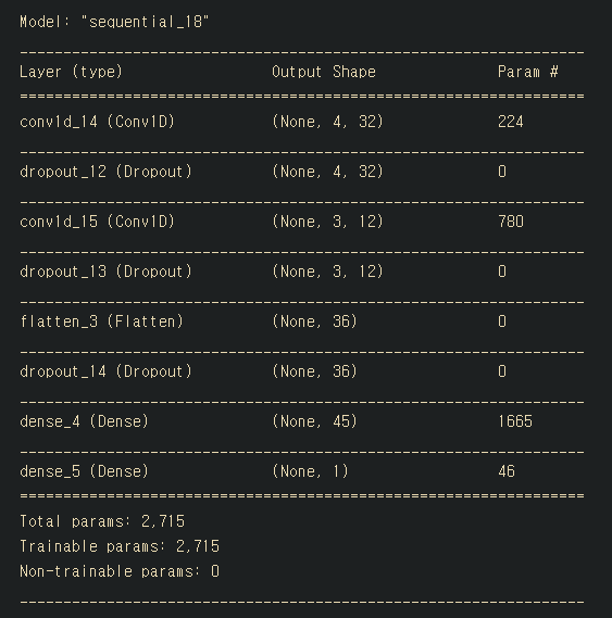
history = model.fit(xtrain, ytrain,epochs=500, verbose=0)
plt.plot(history.history['loss'])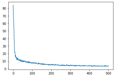
model.evaluate(xtest,ytest)
>>> 3/3 [==============================] - 0s 1ms/step - loss: 7.5618
    7.561756610870361
y_predict=model.predict(xtest)
fig, ax1 = plt.subplots(nrows=1)
fig.set_size_inches(40,10)
ax1.plot(ytest, marker = "o", label = "actual") # 100일간 데이터
ax1.plot(y_predict, marker = "o", label="predict") # 100일간 데이터
ax1.legend(prop={'size':30})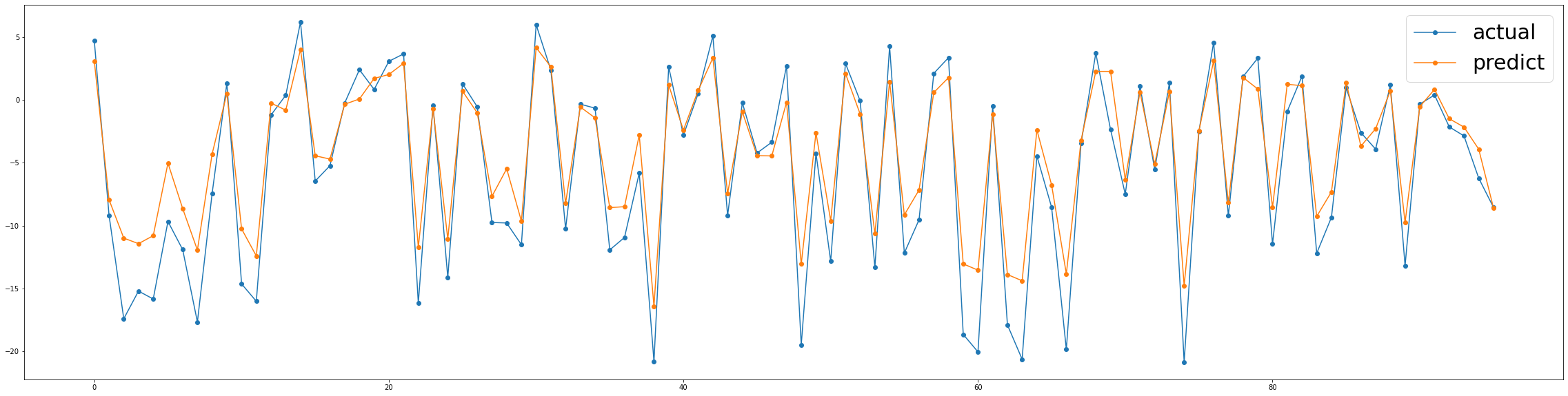
결론
프로세스의 이전 상태를 매 타임 스텝마다 프로세스의 picture로 보는 것은 다변량 시계열 예측을 위한 합리적인 접근방식 처럼 보입니다. 이 접근방식은 재무 시계열 예측, 온도/날씨 예측, 프로세스 변수 모니터링 등 문제의 최고 책임자에게 문제를 구조화할 수 있습니다.
나는 여전히 결과를 개선하기 위해 windows와 picture를 만드는 새로운 방법에 대해서 생각해보고 싶지만, 내가 보기엔, 우리가 다 해보고 나서 볼 수 있듯이, 결코 실제 값을 넘어서지 않는 견고한 모듈 처럼 보입니다.
나는 당신이 이를 개선하기 위해 무엇을 생각해냈는지 많이 알고싶네요!
CNN 부분은 코드가 있지않아 직접 작성해보았습니다.
여러 시계열 예측을 해본 결과 가우시안 프로세스가 가장 낮은 RMSE 값을 가져왔네요,
혹시 오역이나 문제가될 사항이 있다면 문의를 댓글로 남겨주세요!
'노트 > Python : 프로그래밍' 카테고리의 다른 글
| Keras와 OpenCV를 활용하여 웹캠으로 실시간 나이, 성별, 감정 예측 (번역) (3) | 2021.03.26 |
|---|---|
| [시계열] 케라스에서 Luong 어텐션을 활용한 seq2seq2 LSTM 모델 만들기 (번역) (4) | 2020.12.16 |
| [Pandas] Pandas를 마스터하기 위한 30가지 예제 (0) | 2020.11.09 |
| [CS] 이진탐색트리(Binary Search Tree) 구현하기 python code (0) | 2020.11.03 |
| [가상환경] conda 가상환경 명령어 (0) | 2020.10.15 |