2020. 11. 9. 13:38ㆍ노트/Python : 프로그래밍
30 Examples to Master Pandas
A comprehensive practical guide for learning Pandas

Pandas is a widely-used data analysis and manipulation library for Python. It provides numerous functions and methods that expedite the data analysis and preprocessing steps.
Due to its popularity, there are lots of articles and tutorials about Pandas. This one will be one of them but heavily focusing on the practical side. I will do examples on a customer churn dataset that is available on Kaggle.
The examples will cover almost all the functions and methods you are likely to use in a typical data analysis process.
Let’s start by reading the csv file into a pandas dataframe.
import numpy as np
import pandas as pddf = pd.read_csv("/content/churn.csv")

df.shape
(10000,14)

df.columns
Index(['RowNumber', 'CustomerId', 'Surname', 'CreditScore', 'Geography', 'Gender', 'Age', 'Tenure', 'Balance', 'NumOfProducts', 'HasCrCard','IsActiveMember','EstimatedSalary', 'Exited'], dtype='object')
1. Dropping columns
The drop function is used to drop columns and rows. We pass the labels of rows or columns to be dropped.
df.drop(['RowNumber', 'CustomerId', 'Surname', 'CreditScore'], axis=1, inplace=True)

df.shape
(10000,10)
The axis parameter is set as 1 to drop columns and 0 for rows. The inplace parameter is set as True to save the changes. We dropped 4 columns so the number of columns reduced to 10 from 14.
2. Select particular columns while reading
We can read only some of the columns from the csv file. The list of columns is passed to the usecols parameter while reading. It is better than dropping later on if you know the column names beforehand.
df_spec = pd.read_csv("/content/churn.csv", usecols=['Gender', 'Age', 'Tenure', 'Balance'])
df_spec.head()
(image by author)
3. Reading a part of the dataframe
The read_csv function allows reading a part of the dataframe in terms of the rows. There are two options. The first one is to read the first n number of rows.
df_partial = pd.read_csv("/content/churn.csv", nrows=5000)

df_partial.shape
(5000,14)
Using the nrows parameters, we created a dataframe that contains the first 5000 rows of the csv file.
We can also select rows from the end of the file by using the skiprows parameter. Skiprows=5000 means that we will skip the first 5000 rows while reading the csv file.
4. Sample
After creating a dataframe, we may want to draw a small sample to work. We can either use the n parameter or frac parameter to determine the sample size.
- n: The number of rows in the sample
- frac: The ratio of the sample size to the whole dataframe size
df_sample = df.sample(n=1000)
df_sample.shape
(1000,10)

df_sample2 = df.sample(frac=0.1)
df_sample2.shape
(1000,10)
5. Checking the missing values
The isna function determines the missing values in a dataframe. By using the isna with the sum function, we can see the number of missing values in each column.
df.isna().sum()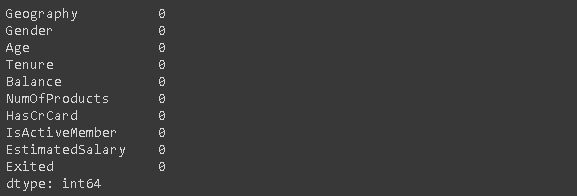
(image by author)
There are no missing values.
6. Adding missing values using loc and iloc
I’m doing this example to practice the “loc” and “iloc”. These methods select rows and columns based on index or label.
- loc: selects with label
- iloc: selects with index
Let’s first create 20 random indices to select.
missing_index = np.random.randint(10000, size=20)We will use these indices to change some values as np.nan (missing value).
df.loc[missing_index, ['Balance','Geography']] = np.nanThere are 20 missing values in the “Balance” and “Geography” columns. Let’s do another example using the indices instead of labels.
df.iloc[missing_index, -1] = np.nan“-1” is the index of the last column which is “Exited”.
Although we’ve used different representations of columns for loc and iloc, row values have not changed. The reason is that we are using numerical index labels. Thus, both label and index for a row are the same.
The number of missing values have changed:
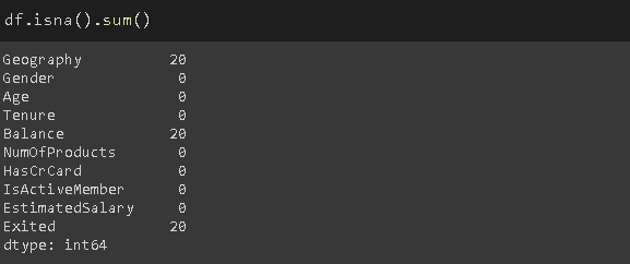
(image by author)
7. Filling missing values
The fillna function is used to fill the missing values. It provides many options. We can use a specific value, an aggregate function (e.g. mean), or the previous or next value.
For the geography column, I will use the most common value.
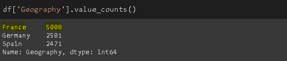
(image by author)
mode = df['Geography'].value_counts().index[0]
df['Geography'].fillna(value=mode, inplace=True)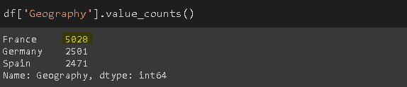
(image by author)
Similarly, for the balance column, I will use the mean of the column to replace missing values.
avg = df['Balance'].mean()
df['Balance'].fillna(value=avg, inplace=True)
The method parameter of the fillna function can be used to fill missing values based on the previous or next value in a column (e.g. method=’ffill’). It can be pretty useful for sequential data (e.g. time series).
8. Dropping missing values
Another way to handle missing values is to drop them. There are still missing values in the “Exited” column. The following code will drop rows that have any missing value.
df.dropna(axis=0, how='any', inplace=True)The axis=1 is used to drop columns with missing values. We can also set a threshold value for the number of non-missing values required for a column or row to have. For instance, thresh=5 means that a row must have at least 5 non-missing values not to be dropped. The rows that have 4 or fewer missing values will be dropped.
The dataframe does not have any missing values now.
df.isna().sum().sum()
0
9. Selecting rows based on conditions
In some cases, we need the observations (i.e. rows) that fit some conditions. For instance, the below code will select customers who live in France and have churned.
france_churn = df[(df.Geography == 'France') & (df.Exited == 1)]
france_churn.Geography.value_counts()

France 808
10. Describing the conditions with query
The query function provides a more flexible way of passing the conditions. We can describe them with strings.
df2 = df.query('80000 < Balance < 100000')Let’s confirm the result by plotting a histogram of the balance column.
df2['Balance'].plot(kind='hist', figsize=(8,5))
(image by author)
11. Describing the conditions with isin
The condition might have several values. In such cases, it is better to use the isin method instead of separately writing the values.
We just pass a list of the desired values.
df[df['Tenure'].isin([4,6,9,10])][:3]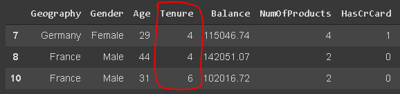
(image by author)
12. The groupby function
Pandas Groupby function is a versatile and easy-to-use function that helps to get an overview of the data. It makes it easier to explore the dataset and unveil the underlying relationships among variables.
We will do several examples of the groupby function. Let’s start with a simple one. The code below will group the rows based on the geography-gender combinations and then give us the average churn rate for each group.
df[['Geography','Gender','Exited']].groupby(['Geography','Gender']).mean()
(image by author)
13. Applying multiple aggregate functions with groupby
The agg function allows applying multiple aggregate functions on the groups. A list of the functions is passed as an argument.
df[['Geography','Gender','Exited']].groupby(['Geography','Gender']).agg(['mean','count'])
(image by author)
We can see both the count of the observations (rows) in each group and the average churn rate.
14. Applying different aggregate functions to different groups
We do not have to apply the same function to all columns. For instance, we may want to see the average balance and the total number of churned customers in each country.
We will pass a dictionary that indicates which functions are to be applied to which columns.
df_summary = df[['Geography','Exited','Balance']].groupby('Geography')\
.agg({'Exited':'sum', 'Balance':'mean'})

df_summary.rename(columns={'Exited':'# of churned customers', 'Balance':'Average Balance of Customers'},inplace=True)
df_summary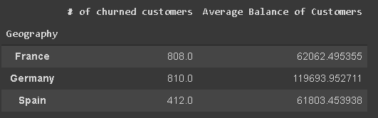
(image by author)
I have also renamed the columns.
Edit: Thanks Ron for the heads-up in the comment section. The NamedAgg function allows renaming the columns in the aggregation. The syntax is as follows:
df_summary = df[['Geography','Exited','Balance']].groupby('Geography')\
.agg(
Number_of_churned_customers = pd.NamedAgg('Exited', 'Sum'),
Average_balance_of_customers = pd.NamedAgg('Balance', 'Mean')
)
15. Reset the index
As you may have noticed, the index of the dataframes that the groupby returns consist of the group names. We can change it by resetting the index.
df_new = df[['Geography','Exited','Balance']]\
.groupby(['Geography','Exited']).mean().reset_index()

df_new
(image by author)
Edit: Thanks Ron for the heads-up in the comment section. If we set the as_index parameter of the groupby function as False, the group names will not be used as the index.
16. Reset the index with a drop
In some cases, we need to reset the index and get rid of the original index at the same time. Consider a case where draw a sample from a dataframe. The sample will keep the index of the original dataframe so we want to reset it.
df[['Geography','Exited','Balance']].sample(n=6).reset_index()
(image by author)
The index is reset but the original is kept as a new column. We can drop it while resetting the index.
df[['Geography','Exited','Balance']]\
.sample(n=6).reset_index(drop=True)
(image by author)
17. Set a particular column as the index
We can set any column in the dataframe as the index.
df_new.set_index('Geography')
(image by author)
18. Inserting a new column
We can add a new column to a dataframe as follows:
group = np.random.randint(10, size=6)
df_new['Group'] = groupdf_new
(image by author)
But the new column is added at the end. If you want to put the new column at a specific position, you can use the insert function.
df_new.insert(0, 'Group', group)
df_new
(image by author)
The first parameter is the index of the location, the second one is the name of the column, and the third one is the value.
19. The where function
It is used to replace values in rows or columns based on a condition. The default replacement value is NaN but we can also specify the value to be put as a replacement.
Consider the dataframe in the previous step (df_new). We want to set the balance to 0 for customers who belong to a group that is less than 6.
df_new['Balance'] = df_new['Balance'].where(df_new['Group'] >= 6, 0)
df_new
(image by author)
The values that fit the specified condition remain unchanged and the other values are replaced with the specified value.
20. The rank function
It assigns a rank to the values. Let’s create a column that ranks the customers according to their balances.
df_new['rank'] = df_new['Balance'].rank(method='first', ascending=False).astype('int')
df_new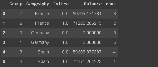
(image by author)
The method parameter specifies how to handle the rows that have the same values. ‘First’ means they are ranked according to their order in the array (i.e. column).
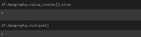
21. Number of unique values in a column
It comes in handy when working with categorical variables. We may need to check the number of unique categories.
We can either check the size of the series returned by the value counts function or use the nunique function.
(image by author)
22. Memory usage
It is simply done by the memory_usage function.
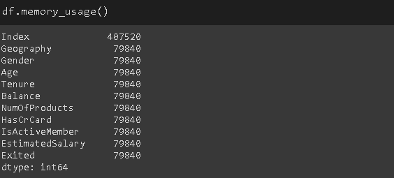
(image by author)
The values show how much memory is used in bytes.
23. The category data type
By default, categorical data is stored with the object data type. However, it may cause unnecessary memory usage especially when the categorical variable has low cardinality.
Low cardinality means that a column has very few unique values compared to the number of rows. For instance, the geography column has 3 unique values and 10000 rows.
We can save memory by changing its data type as “category”.
df['Geography'] = df['Geography'].astype('category')
(image by author)
The memory consumption of the geography column is reduced by almost 8 times.
24. Replacing values
The replace function can be used to replace values in a dataframe.
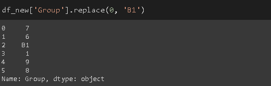
(image by author)
The first parameter is the value to be replaced and the second one is the new value.
We can use a dictionary to do multiple replacements.
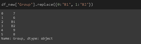
(image by author)
25. Drawing a histogram
Pandas is not a data visualization library but it makes it pretty simple to create basic plots.
I find it easier to create basic plots with Pandas instead of using an additional data visualization library.
Let’s create a histogram of the balance column.
df['Balance'].plot(kind='hist', figsize=(10,6), title='Customer Balance')
(image by author)
I do not want to go into detail about plotting since pandas is not a data visualization library. However, the plot function is capable of creating many different plots such as line, bar, kde, area, scatter, and so on.
26. Reducing the decimal points of floats
Pandas may display an excessive amount of decimal points for floats. We can easily adjust it using the round function.
df_new.round(1) #number of desired decimal points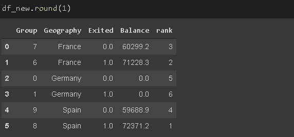
(image by author)
27. Changing the display options
Instead of adjusting the display options manually at each time, we can change the default display options for various parameters.
- get_option: Returns what the current option is
- set_option: Changes the option
Let’s change the display option for decimal points to 2.
pd.set_option("display.precision", 2)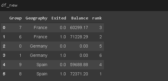
(image by author)
Some other options you may want to change are:
- max_colwidth: Maximum number of characters displayed in columns
- max_columns: Maximum number of columns to display
- max_rows: Maximum number of rows to display
28. Calculating the percentage change through a column
The pct_change is used to calculate the percent change through the values in a series. It is useful when calculating the percentage of change in a time series or sequential array of elements.
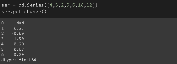
(image by author)
The change from the first element (4) to the second element (5) is %25 so the second value is 0.25.
29. Filtering based on strings
We may need to filter observations (rows) based on textual data such as the name of customers. I’ve added made-up names to the df_new dataframe.
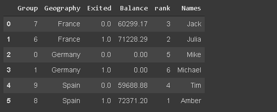
(image by author)
Let’s select the rows in which the customer name starts with ‘Mi’.
We will use the startswith method of the str accessor.
df_new[df_new.Names.str.startswith('Mi')]
(image by author)
The endswith function does the same filtering based on the characters at the end of strings.
There are lots of operations that pandas can do with strings. I have a separate article on this topic if you’d like to read further.
5 Must-Know Pandas Operations on Strings
String manipulation made easy with Pandas
towardsdatascience.com
30. Styling a dataframe
We can achieve this by using the Style property which returns a styler object It provides many options for formatting and displaying dataframes. For instance, we can highlight the minimum or maximum values.
It also allows for applying custom styling functions.
df_new.style.highlight_max(axis=0, color='darkgreen')
(image by author)
I have a detailed post on styling pandas dataframes if you’d like to read further.
Style Your Pandas Dataframes
Let’s create something more than plain numbers.
towardsdatascience.com
Conclusion
We have covered a great deal of the functions and methods for data analysis. There are, of course, a lot more offered by pandas but it is impossible to cover all in one article.
As you keep using pandas for your data analysis tasks, you may discover new functions and methods. As with any other subject, practice makes perfect.
I’d like to share two other posts that kind of cover different operations than the ones in this post.
Thank you for reading. Please let me know if you have any feedback.
출처
towardsdatascience.com/30-examples-to-master-pandas-f8a2da751fa4
30 Examples to Master Pandas
A comprehensive practical guide for learning Pandas
towardsdatascience.com
'노트 > Python : 프로그래밍' 카테고리의 다른 글
| [시계열] 케라스에서 Luong 어텐션을 활용한 seq2seq2 LSTM 모델 만들기 (번역) (4) | 2020.12.16 |
|---|---|
| [시계열] Time Series에 대한 머신러닝(ML) 접근 (2) | 2020.12.12 |
| [CS] 이진탐색트리(Binary Search Tree) 구현하기 python code (0) | 2020.11.03 |
| [가상환경] conda 가상환경 명령어 (0) | 2020.10.15 |
| [신경망] LSTM 모델을 이용한 리뷰 요약하기 (2) | 2020.05.20 |